Millionaire Odds vs. Hit by a Bus: An ES|QL Analysis

ES|QL is designed for fast, efficient querying of large datasets. It has a straightforward syntax which will allow you to write complex queries easily, with a pipe based language, reducing the learning curve. We're going to use ES|QL to run statistical analysis and compare different odds.

If you are reading this, you probably want to know how rich you can get before actually reaching the same odds of being hit by a bus. I can't blame you, I want to know too. Let's work out the odds so that we can make sure we win the lottery rather than get in an accident!

What we are going to see in this blog is figuring out the probability of being hit by a bus and the probability of achieving wealth. We'll then compare both and understand until what point your chances of getting rich are higher, and when you should consider getting life insurance.

So how are we going to do that? This is going to be a mix of magic numbers pulled from different articles online, some synthetics data and the power of ES|QL, the new Elasticsearch Query Language. Let's get started.

The Data

The magic number

The challenge starts here as the dataset is going to be somewhat challenging to find. We are then going to assume for the sake of the example that ChatGPT is always right. Let’s see what we get for the following question:

Cough Cough… That sounds about right, this is going to be our magic number.

Generating the wealth data

Prerequisites

Before running any of the scripts below, make sure to install the following packages:

elasticsearch==8.14.0
matplotlib
numpy
panda
scipy

Now, there is one more thing we need, a representative dataset with wealth distribution to compute wealth probability. There is definitely some portion of it here and there, but again, for the example we are going to generate a 500K line dataset with the below python script. I am using python 3.11.5 in this example:

import pandas as pd
import numpy as np
import getpass
from elasticsearch import Elasticsearch, helpers

# Input the Elasticsearch host
hosts = input('Enter your Elasticsearch host address : ')

# Securely input the Elasticsearch API key
api_key = getpass.getpass(prompt='Enter your Elasticsearch API Key: ')

# Initialize Elasticsearch client
client = Elasticsearch(
    hosts=hosts,
    api_key=api_key,
)

# Generate synthetic data with a highly skewed distribution
num_records = 500000
np.random.seed(42)  # Ensure reproducibility

# Generate net worth using a highly skewed distribution
ages = np.random.randint(20, 80, num_records)  # Random ages between 20 and 80
incomes = np.random.exponential(scale=10000, size=num_records)  # Exponential distribution for income
# Use a more skewed distribution for net worth with a much larger range
net_worths = np.random.exponential(scale=100000000, size=num_records)  # Extremely skewed net worth

# Scale up the net worths to reach up to $100 billion
net_worths = np.clip(net_worths, 0, 100000000000)

# Create DataFrame
df = pd.DataFrame({
    'id': range(1, num_records + 1),
    'age': ages,
    'income': incomes,
    'net_worth': net_worths,
    'counter': range(1, num_records + 1)  # Add a counter field for pagination
})

# Index the data into Elasticsearch
index_name = 'raw_wealth_data_large'
try:
    if client.indices.exists(index=index_name):
        client.indices.delete(index=index_name)
except exceptions.NotFoundError:
    pass
client.indices.create(index=index_name)


def generator(df):
    for index, row in df.iterrows():
        yield {
            "_index": index_name,
            "_source": row.to_dict()
        }

helpers.bulk(client, generator(df))

print("Data indexed successfully.")

It should take some time to run depending on your configuration since we are injecting 500K documents here!

FYI, after playing with a couple of versions of the script above and the ESQL query on the synthetic data, it was obvious that the net worth generated across the population was not really representative of the real world. So I decided to use a log-normal distribution (np.random.lognormal) for income to reflect a more realistic spread where most people have lower incomes, and fewer people have very high incomes.

Net Worth Calculation: Used a combination of random multipliers (np.random.uniform(0.5, 5)) and additional noise (np.random.normal(0, 10000)) to calculate net worth. Added a check to ensure no negative net worth values by using np.maximum(0, net_worths).

Not only have we generated 500K documents, but we also used the Elasticsearch python client to bulk ingest all these documents in our deployment. Please note that you will find the endpoint to pass in as hosts Cloud ID in the code above.

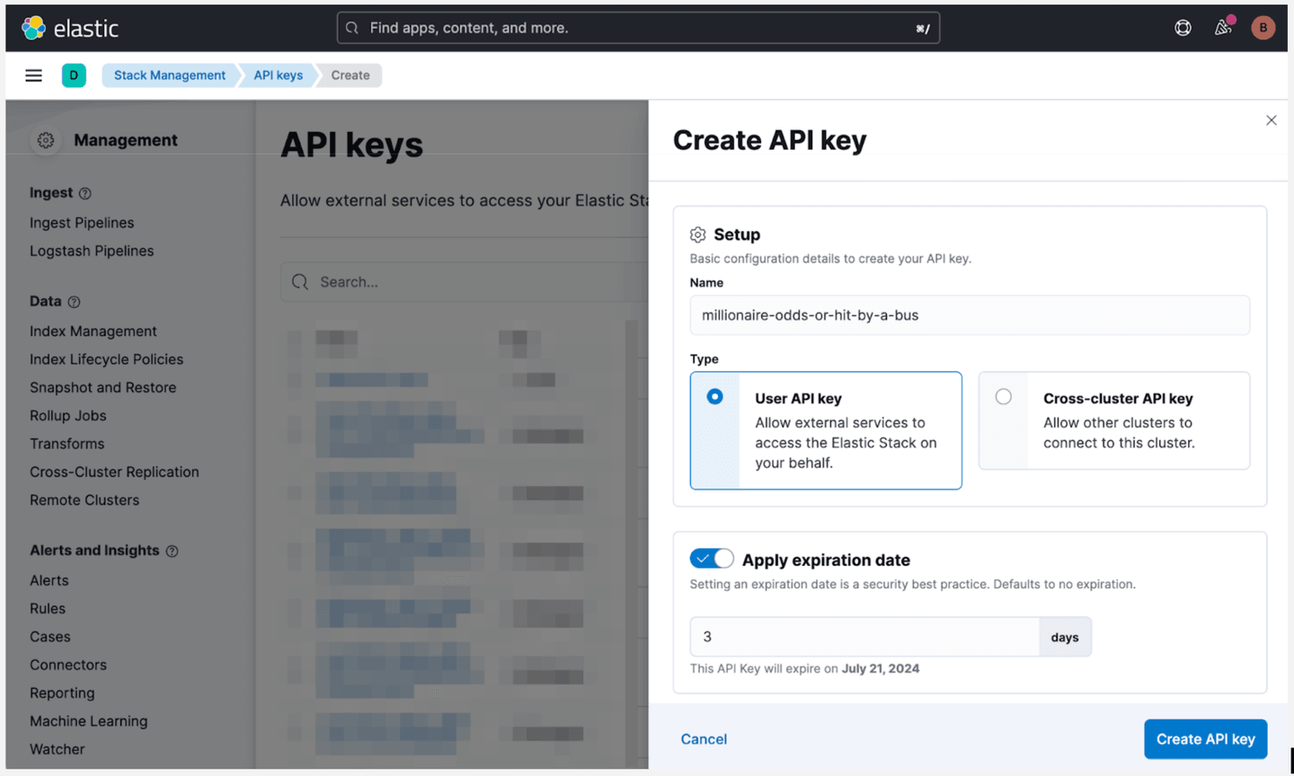
For the deployment API key, open Kibana, and generate the key in Stack Management / API Keys:

The good news is that if you have a real data set, all you will need to do is to change the above code to read your dataset and write documents with the same data mapping.

Ok we're getting there! The next step is pouring our wealth distribution.

ES|QL Wealth Analysis

Introducing ES|QL: A Powerful Tool for Data Analysis

The arrival of Elasticsearch Query Language (ES|QL) is very exciting news for our users. It largely simplifies querying, analyzing, and visualizing data stored in Elasticsearch, making it a powerful tool for all data-driven use cases.

ES|QL comes with a variety of functions and operators, to perform aggregations, statistical analyses, and data transformations. We won’t address them all in this blog post, however our documentation is very detailed and will help you familiarize with the language and the possibilities.

To get started with ES|QL today and run the blog post queries, simply start a trial on Elastic Cloud, load the data and run your first ES|QL query.

Understanding the wealth distribution with our first query

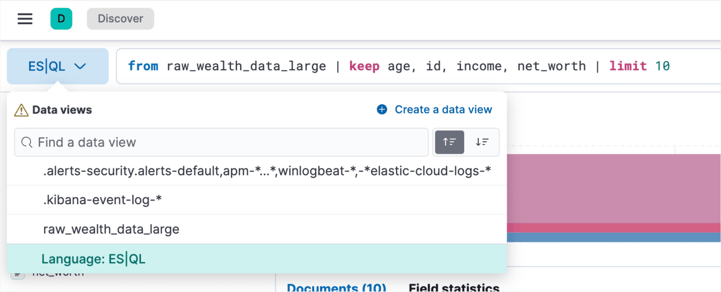
To get familiar with the dataset, head to Discover in Kibana and switch to ES|QL in the dropdown on the left hand side:

Let’s fire our first request:

from raw_wealth_data_large | keep age, id, income, net_worth | limit 10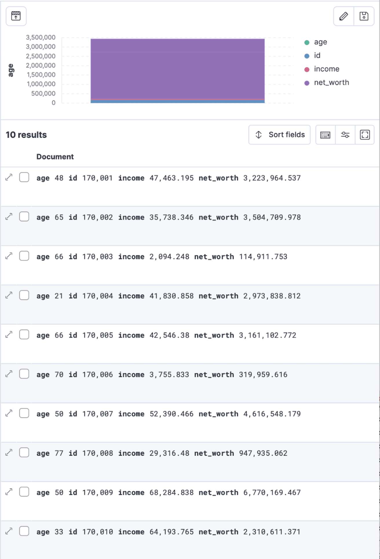

As you could expect from our indexing script earlier, we are finding the documents we bulk ingested, notice the simplicity of pulling data from a given dataset with ES|QL where every query starts with the From clause, then your index.

In the query above given we have 500K lines, we limited the amount of returned documents to 10. To do this, we are passing the output of the first segment of the query via a pipe to the limit command to only get 10 results. Pretty intuitive, right?

Alright, what would be more interesting is to understand the wealth distribution in our dataset, for this we will leverage one of the 30 functions ES|QL provides, namely percentile.

This will allow us to understand the relative position of each data point within the distribution of net worth. By calculating the median percentile (50th percentile), we can gauge where an individual’s net worth stands compared to others.

FROM raw_wealth_data_large
| stats p50 = percentile(net_worth, 50)

Like our first query, we are passing the output of our index to another function, Stats, which combined with the percentile function will output the median net worth:

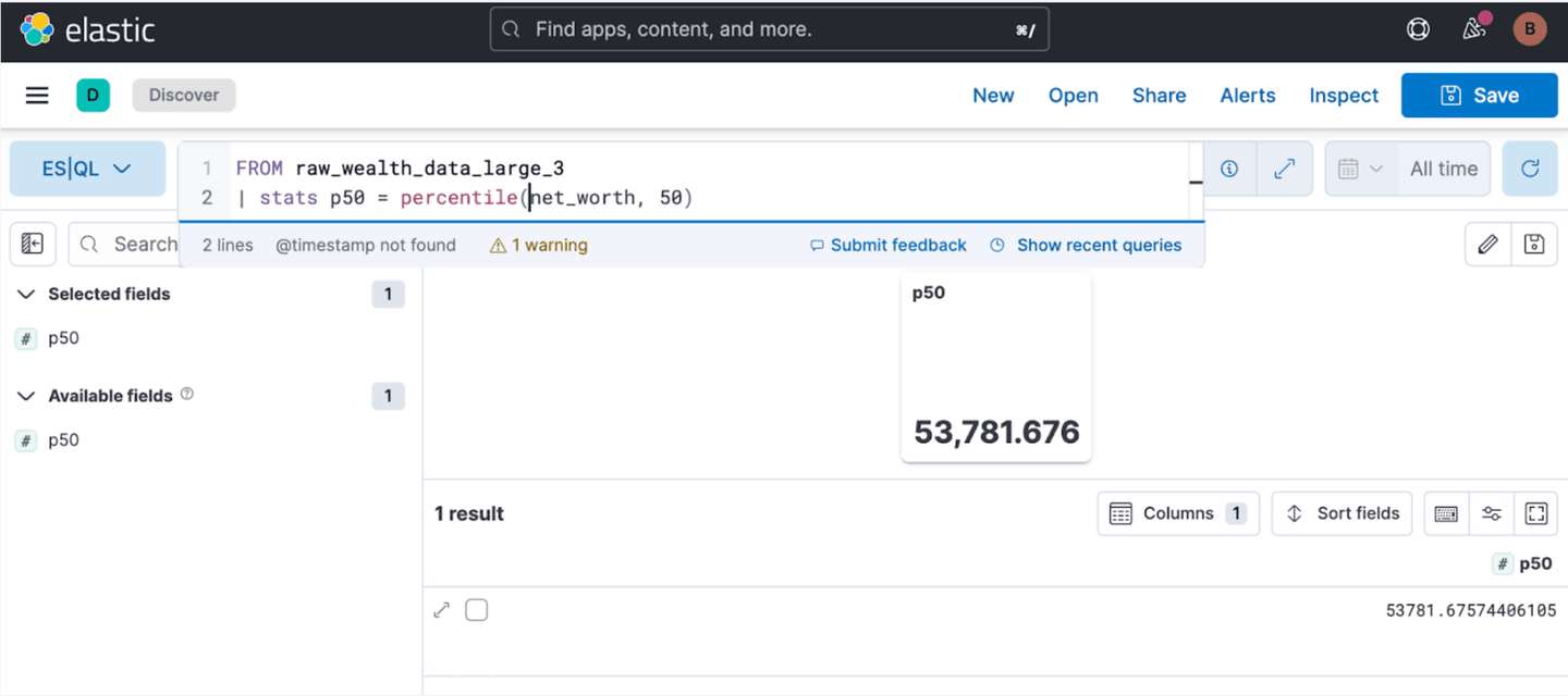
The median is about 54K, which unfortunately is probably optimistic compared to the real world, but we are not going to solve this here. If we go a little further, we can look at the distribution in more granularity by computing more percentiles:

FROM raw_wealth_data_large
| STATS  p25 = percentile(net_worth, 25)
       , p50 = percentile(net_worth, 50)
       , p75 = percentile(net_worth, 75)
       , p90 = percentile(net_worth, 90)
       , p95 = percentile(net_worth, 95)
       , p96 = percentile(net_worth, 96)
       , p98 = percentile(net_worth, 98)
       , p97 = percentile(net_worth, 97)
       , p99 = percentile(net_worth, 99)
| keep p25, p25, p50, p75, p90, p95, p96, p97, p98, p99

With the below output:

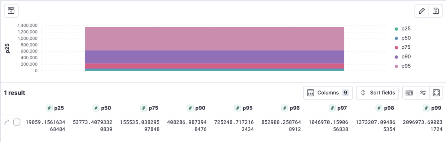
The data reveals a significant disparity in wealth distribution, with the majority of wealth being concentrated among the richest individuals. Specifically, the top 5% (95th percentile) possess a disproportionately large portion of the total wealth, with a net worth starting at $852,988.26 and increasing dramatically in the higher percentiles.

The 99th percentile individuals hold a net worth exceeding $2 million, highlighting the skewed nature of wealth distribution. This indicates that a substantial portion of the population has modest net worth, which is probably what we want for this example.

Another way to look at this is to augment the previous query and grouping by age to see if there is, (in our synthetic dataset), a relation between wealth and age:

FROM raw_wealth_data_large
| STATS  p25 = percentile(net_worth, 25)
      , p50 = percentile(net_worth, 50)
      , p75 = percentile(net_worth, 75)
      , p90 = percentile(net_worth, 90)
      , p95 = percentile(net_worth, 95)
      , p96 = percentile(net_worth, 96)
      , p98 = percentile(net_worth, 98)
      , p97 = percentile(net_worth, 97)
      , p99 = percentile(net_worth, 99) by age
| keep p25, p25, p50, p75, p90, p95, p96, p97, p98, p99, age

This could be visualized in a Kibana dashboard. Simply:

• Navigate to Dashboard
• Add a new ES|QL visualization
• Copy and paste our query
• Move the age field to the horizontal axis in the visualization configuration

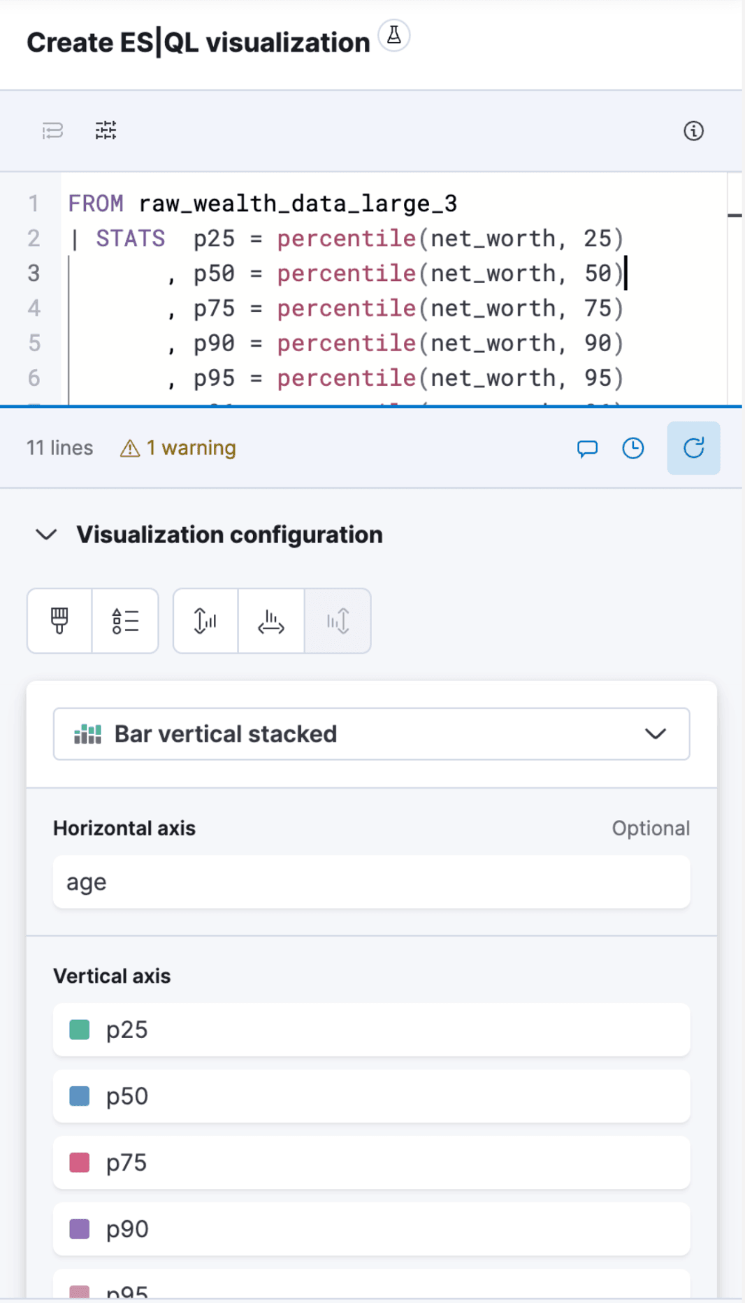
Which will output:

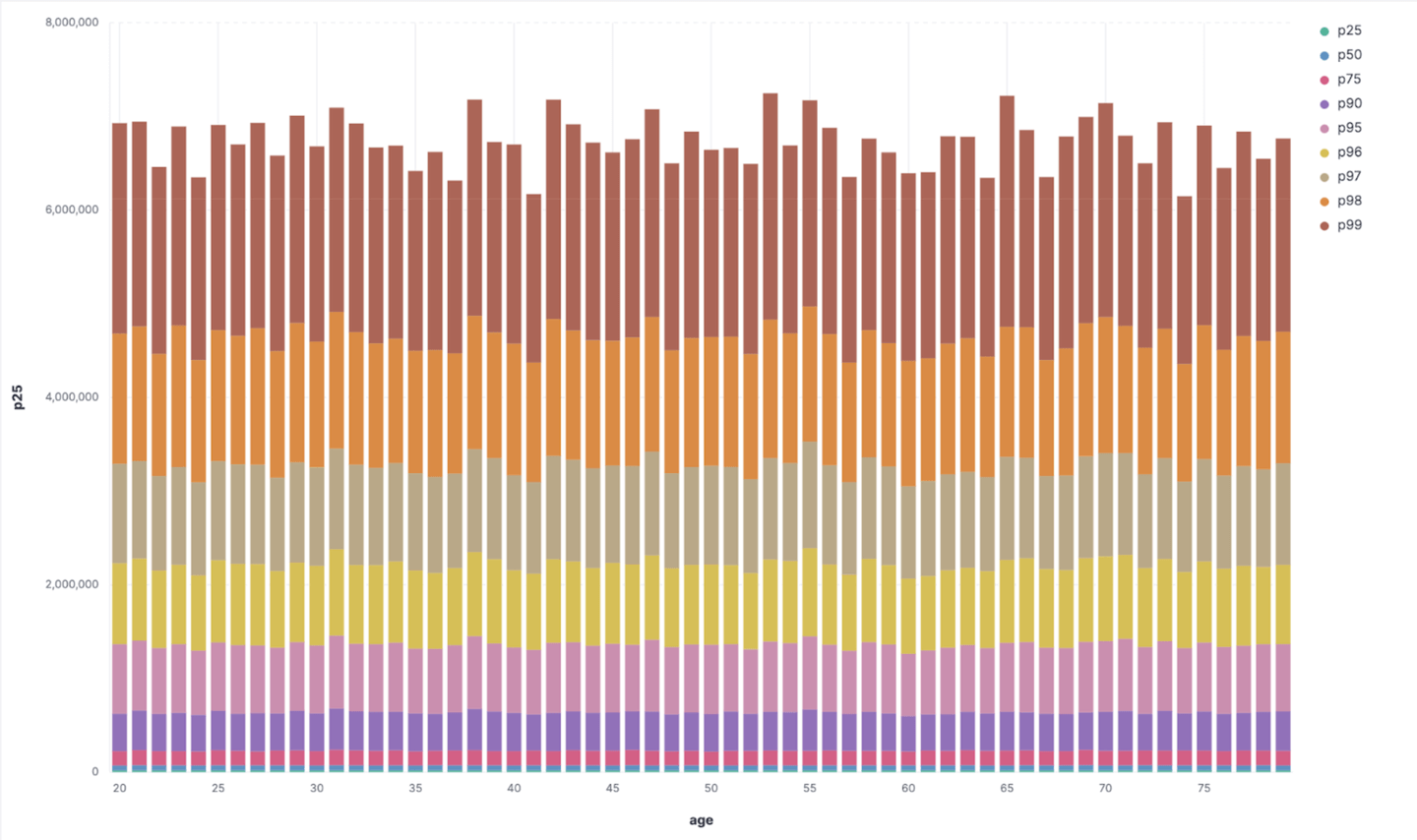
The above suggests that the data generator randomized wealth uniformly across the population age, there is no specific trend pattern we can really see.

Median Absolute Deviation (MAD)

We calculate the median absolute deviation (MAD) to measure the variability of net worth in a robust manner, less influenced by outliers.

FROM raw_wealth_data_large
| stats median_net_worth = MEDIAN(net_worth), mad_net_worth = MEDIAN_ABSOLUTE_DEVIATION(net_worth)
| keep median_net_worth, mad_net_worth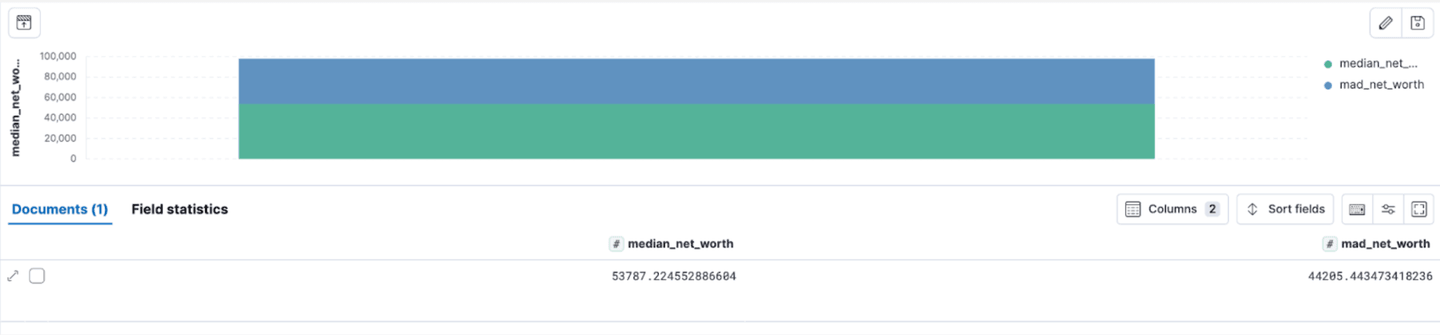

With a median net worth of $53,787.22 and a MAD of$44,205.44, we can infer the typical range of Net Worth: Most individuals’ net worth falls within a range of $44,205.44 above and below the median. This gives a typical range of approximately$9,581.78 to $97,992.66.

The statistical showdown between Net Worth and Bus Collision

Alright, this is the moment to understand how rich we can get, based on our dataset, before getting hit by a bus. To do that, we are going to leverage ES|QL to pull our entire dataset in chunks and load it into a pandas dataframe to build a net worth probability distribution. Finally, we will determine where the ends meet between the net worth and bus collision probabilities.

The entire Python notebook is available here. I also recommend you read this blog post which walks you through using ES|QL with pandas dataframes.

Helper functions

As you can see in the previously referred blog post, we introduced support for ES|QL since version 8.12 of the Elasticsearch python client. Thus our notebook first defines the below functions:

from io import StringIO

# Function to execute ESQL query and fetch data in chunks
def execute_esql_query(query):
    response = client.esql.query(query=query, format="csv")
    return pd.read_csv(StringIO(response.body))

# Function to fetch paginated data using the counter field
def fetch_paginated_data(index, num_records, size=10000):
    all_data = pd.DataFrame()
    for start in range(1, num_records + 1, size):
        end = start + size - 1
        query = f"""
        FROM {index}
        | WHERE counter >= {start} AND counter <= {end}
        | limit {size}
        """
        data_chunk = execute_esql_query(query)
        all_data = pd.concat([all_data, data_chunk], ignore_index=True)
    return all_data

The first function is straightforward and executes an ES|QL query, the second is fetching the entire dataset from our index. Notice the trick in there that I am using a counter built-in to a field in my index to paginate through the data. This is workaround I am using while our engineering team is working on the support for pagination in ES|QL.

Next, knowing that we have 500K documents in our index, we simply call these function to load the data in a data frame:

# Fetch all data using pagination and ES|QL
num_records = 500000
all_data_df = fetch_paginated_data(index_name, num_records)
print(f"Total Data Retrieved: {len(all_data_df)} records")

Fit Pareto distribution

Next, we fit our data to a Pareto distribution, which is often used to model wealth distribution because it reflects the reality that a small percentage of the population controls most of the wealth. By fitting our data to this distribution, we can more accurately represent the probabilities of different net worth levels.

from scipy.stats import pareto



# Fit a Pareto distribution to the data
shape, loc, scale = pareto.fit(all_data_df['net_worth'], floc=0)

# Calculate the probability density for each net worth
all_data_df['net_worth_probability'] = pareto.pdf(all_data_df['net_worth'], shape, loc=loc, scale=scale)

# Normalize the probabilities to sum to 1
all_data_df['net_worth_probability'] /= all_data_df['net_worth_probability'].sum()

print("Data with Net Worth Probability:")
print(all_data_df.head())

We can visualize the pareto distribution with the code below: ``

import matplotlib.pyplot as plt
from scipy.stats import pareto

# Assuming all_data_df contains the fetched net worth data from Elasticsearch
# Fit a Pareto distribution to the data
shape, loc, scale = pareto.fit(all_data_df['net_worth'], floc=0)

# Plot the Net Worth Probability Distribution
plt.figure(figsize=(10, 6))

# Plot histogram of empirical net worth data
plt.hist(all_data_df['net_worth'], bins=100, density=True, alpha=0.6, color='g', label='Empirical Data')

# Plot fitted Pareto distribution
xmin, xmax = plt.xlim()
x = np.linspace(xmin, xmax, 100)
p = pareto.pdf(x, shape, loc=loc, scale=scale)
plt.plot(x, p, 'k', linewidth=2, label='Fitted Pareto Distribution')

# Show the plot
plt.xlabel('Net Worth')
plt.y bnblabel('Probability')
plt.title('Net Worth Probability Distribution')
plt.legend()
plt.grid(True)
plt.show()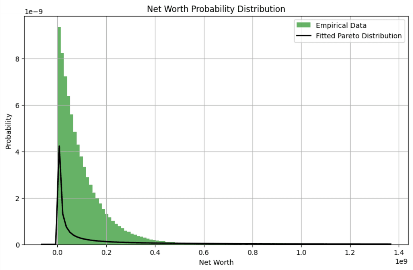

Breaking point

Finally, with the calculated probability, we determine the target net worth corresponding to the bus hit probability and visualize it. Remember, we use the magic number ChatGPT gave us for the probability of getting hit by a bus:

# Find the Net Worth Corresponding to the Bus Hit Probability
target_probability = 0.0000181
cumulative_probability = all_data_df['net_worth_probability'].cumsum()
target_net_worth_df = all_data_df[cumulative_probability >= target_probability].head(1)
target_net_worth = target_net_worth_df['net_worth'].iloc[0]
print(f"Net Worth with Probability >= {target_probability}: {target_net_worth}")

# Plot the Net Worth Probability Distribution
plt.figure(figsize=(10, 6))
plt.hist(all_data_df['net_worth'], bins=100, density=True, alpha=0.6, color='g', label='Empirical Data')
xmin, xmax = plt.xlim()
x = np.linspace(xmin, xmax, 100)
p = pareto.pdf(x, shape, loc=loc, scale=scale)
plt.plot(x, p, 'k', linewidth=2, label='Fitted Pareto Distribution')
plt.axhline(y=target_probability, color='r', linestyle='--', label='Bus Hit Probability')
plt.axvline(x=target_net_worth, color='g', linestyle='--', label=f'Net Worth = {target_net_worth:.2f}')
plt.xlabel('Net Worth')
plt.ylabel('Probability')
plt.title('Net Worth Probability Distribution')
plt.legend()
plt.grid(True)
plt.show()

Conclusion

Based on our synthetic dataset, this chart vividly illustrates that the probability of amassing a net worth of approximately $12.5 million is as rare as the chance of being hit by a bus.

For the fun of it, let’s ask ChatGPT what the probability is:

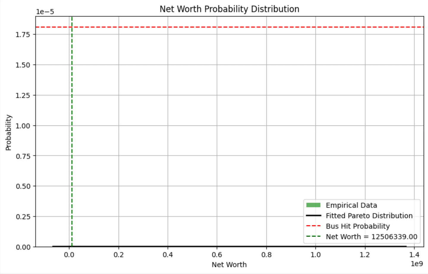
Okay… $439 million? I think ChatGPT might be hallucinating again.