This long-form article explains how generative AI works, from the ground all the way up to generative transformer architectures. The focus is on intuitions, not rigor. A number of technical details are of course simplified. It is a gentle introduction, not a scientific article.
We are breaking it down to two parts: This first part explains how AI understands natural language. This includes embeddings, language models, transformer-encoders, self-attention, fine tuning for AI search and NLP. The second part will build on this to explain how AI uses this understanding to generate text such as responses to your natural language prompts and translations, including decoder-only and full transformer architectures, large language models (LLMs) and retrieval augmented generation (RAG), a prominent generative pattern at which Elastic excels. Because the language models we will discuss involve neural networks, a basic understanding of the neural networks fundamentals is assumed for certain parts in this journey.
The semantic stage of GenAI: Understanding natural language
1. Understanding embeddings, vector similarity and language models
The fundamental construct with which AI understands language is vectors. Vectors represent words and are simply long arrays of numerical values. Technically, vectors may also represent sequences of words or sub-word parts, and so we abstract this with the term tokens (this is not of essence for our discussion and we will be using the terms words and tokens interchangeably).
On the simplest level each word (or token) in a language has a vector representation, i.e. a long array of learned numerical values. You may come across language like “vectors of thousands” or even “tens of thousands of dimensions” but, there is really nothing exotic and please avoid the rabbit hole of squeezing your brain to grasp what “thousands of dimensions” may mean. For each word, each dimension is simply a specific position in this word’s vector and that’s that. We will visualize what this means very shortly and it will become transparent.
Depending on the architecture of the model that is used to represent text, a sparse model will use high dimensional vectors (vectors with 10,000 up to 100 000+ of dimensions) with few non-zero values that are called sparse vectors. In a sparse vector each dimension corresponds to a word in the vocabulary. A vocabulary is the set of all unique words that a model can accept, i.e. they existed in the natural language corpus that the model was trained on (we will see how models are trained in the next sections). So, a sparse vector has as many dimensions as the words in the vocabulary, i.e. tens or hundreds of thousands of dimensions. To simplify the discussion, we will assume 30,000 words in a vocabulary (that's a good approximation of a native English speaker vocabulary on average). In a sparse vector most dimensions hold value zero and a few are non-zero.
In contrast a dense vector has a few hundreds to a few thousands of dimensions which generally hold non-zero values. In dense representations, these numerical values are computed so that semantically relevant words have similar vector representations, i.e. they have similar numerical values in the corresponding position (in other words, they have similar values across each dimension). And you now have the most fundamental description of a starter language model: a simple language model is an assignment of vector values for each word in a language so that semantically related words have similar representations. The more related the words are, the more similar are their vectors. Vector similarity is at the heart of AI.
A convenient thing with vectors is that we can measure their similarity. We do that using distance functions but in the rest of this discussion we will explore vector similarity visually for the concepts to become crystal clear. So to continue the previous reasoning, a language model produces a representation of words in a vector space, such that relevant words have similar vectors i.e. vectors with a small distance between them in the vector space. If this reads a little cryptic, rest assured that we will unpack it in the following paragraphs using intuitive realistic visualizations.
One of the most fundamental ways to produce vector representations and a natural starting point is an algorithm called word2vec (we’ll examine word2vec in detail in the next section). In a word2vec implementation each vector has 300 dimensions. Each of the 300 vector positions holds a value between -1 and +1. Because of the low dimensionality relative to the number of words in the vocabulary and because most of the vector’s positions hold a non-zero value, the word2vec vectors are dense. These dense vectors are also called word embeddings and the word2vec embedding algorithm that produces them is called an embeddings model.
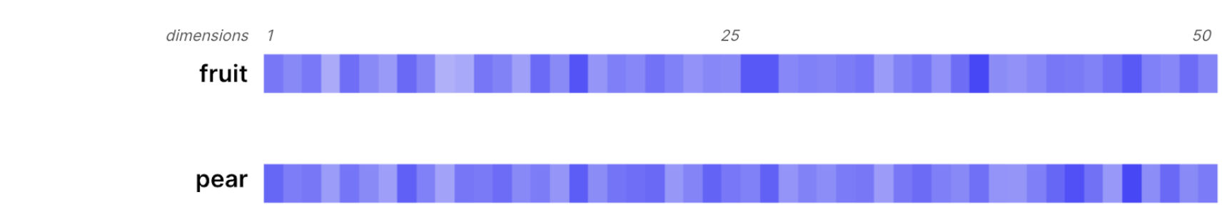
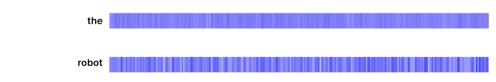
It’s time to visualize these dense vectors, as promised. For quick, naked eye vector similarity, we will represent the values with colors. Blue for -1, white for +1 and corresponding shades of blue for all the values between -1 and +1.
In the visualizations that follow, we are only showing the first 50 positions out of the 300 total, for easier visual comparison of the vectors. Notice the similarity between them.
 |
|---|
| Figure 1. Word2vec vectors (embeddings) for ‘fruit’ and ‘pear’ visually (first 50 of 300 dimensions). Created with Gensim’s trained word2vec and Matplotlib. |
 |
|---|
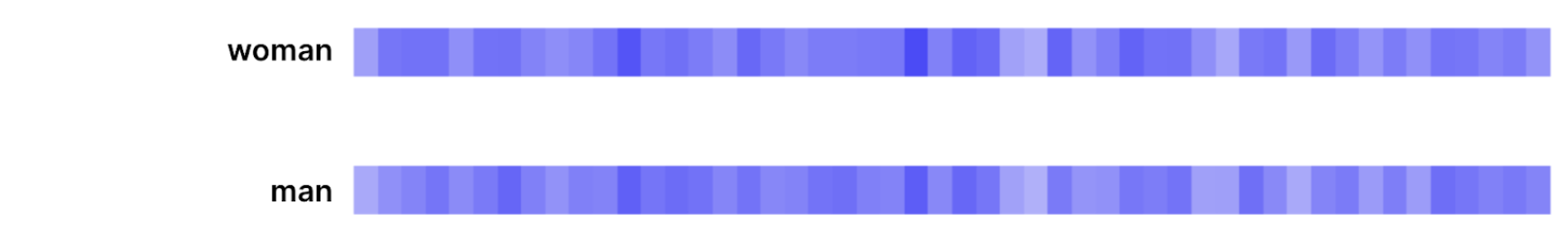
| Figure 2. Word2vec vectors (embeddings) for ‘woman’ and ‘man’ visually (first 50 of 300 dimensions). |
Here is the first crucial point: Vector similarity captures semantic relevance. In the first examples, ‘fruit’ and ‘pear’ are related and ‘man’ and ‘woman’ are related. They are not similar the way synonyms are. Relevance is broader.
 |
|---|
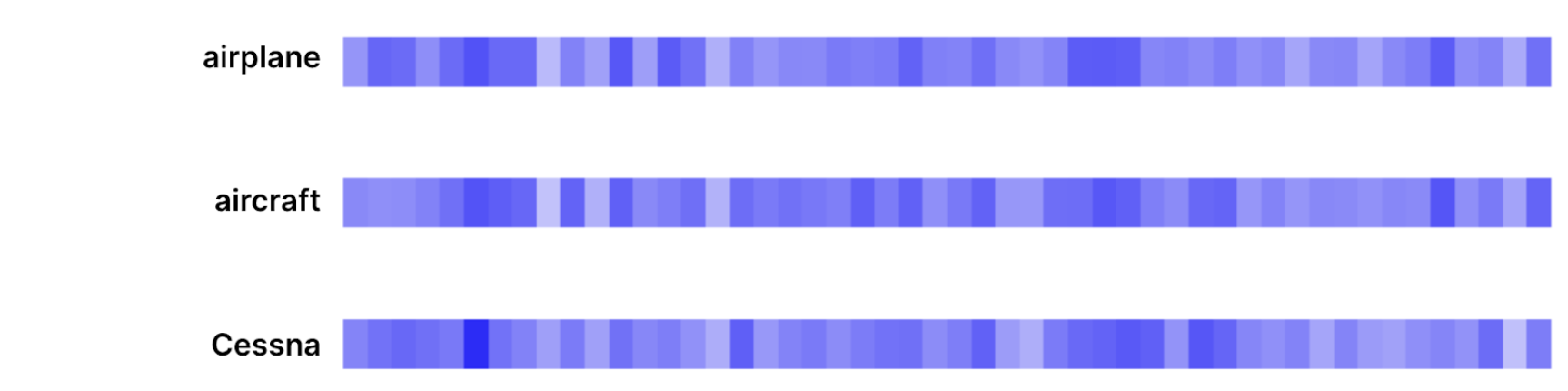
| Figure 3. Word2vec vectors (embeddings) for ‘airplane’, ‘aircraft’ and ‘Cessna’ visually (first 50 of 300 dimensions). |
It is more granular too. Here’s the second crucial point: AI resolves relationships between words and concepts. It does not understand meanings, but it models the relationships between meanings! The closer the relationship, the more similar the vectors, with synonyms being at the end of the spectrum.
A quick note on language: This is the prism through which any reference to "AI understanding language" should be interpreted, in this text and elsewhere. This language should not imply human level understanding. This fact is coined as "the barrier of meaning".
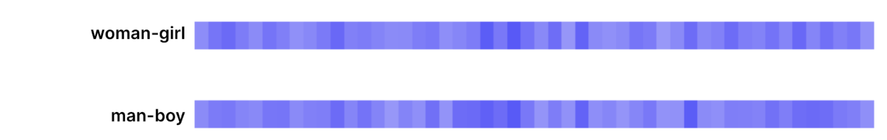
Let’s dig just one level deeper: You are probably wondering how these values (the vector elements) are computed, as there are surely infinite ways that related words have similar vector representations. Dense vector elements are computed during training in a manner that relationships between words are captured (training a language model is a big part of our discussion next). For example a girl is to a woman what a boy is to a man and so, hopefully the delta between ‘woman’ and ‘girl’ is similar to the delta between ‘man’ and ‘boy’.
 |
|---|
| Figure 4. A ‘girl’ is to a ‘woman’ what a ‘boy’ is to a ‘man’. Notice that the delta vectors are similar too (‘Woman’ minus ‘girl’ vs ‘man’ minus ‘boy’). |
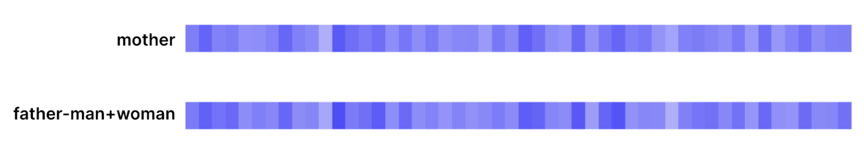
And to stretch it a bit more, if you subtract ‘man’ from ‘father’ and add ‘woman’ you get a vector similar to ‘mother’.
 |
|---|
| Figure 5. ‘Mother’ vs ‘father’ minus ‘man’ plus ‘woman’. |
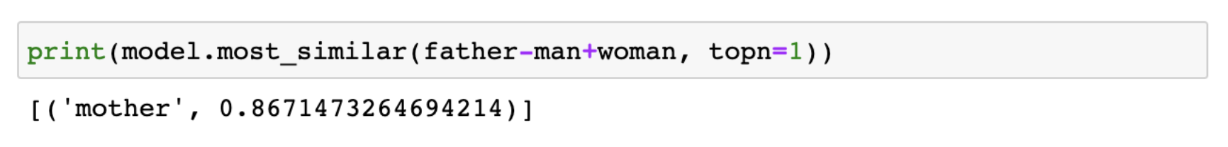
In fact, using Gensim’s most_similar, we can confirm that the most similar vector to the ‘father-man+woman’ vector is actually ‘mother’:
 |
|---|
| Figure 6. ‘Mother’ is the most similar vector to ‘father’ minus ‘man’ plus ‘woman’. |
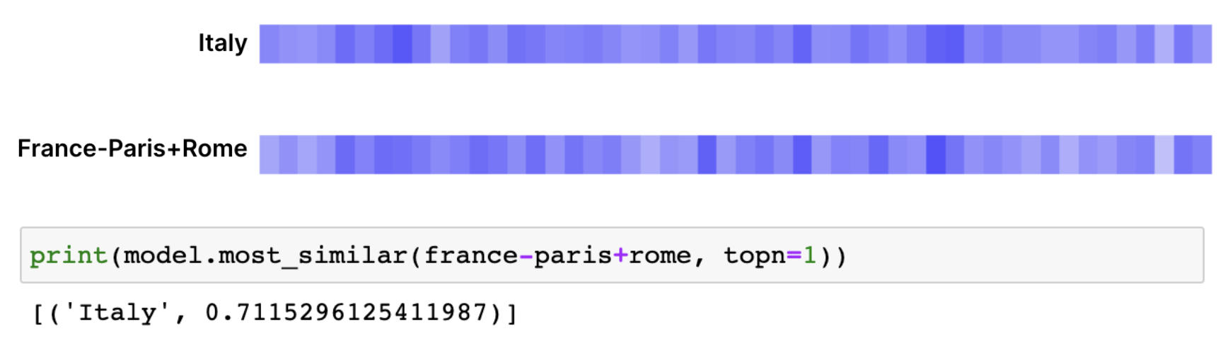
Similarly if you subtract ‘Paris’ from ‘France’ and add ‘Rome’, the most similar vector is 'Italy'.
 |
|---|
| Figure 7. “Italy” vs “France minus Paris plus Rome”. |
The main intuition is that semantic relationships are reflected in certain patterns in the dense vectors. When you train a language model, you are shaping the vector space to reflect the relationships between the words in a language, so that these relationships are captured through the element allocations that you end up with for all dense vectors.
To reinforce this intuition, let’s visualize a semantically “neutral” word like ‘the’ and compare it to a more specific word. In this case, let’s visualize all 300 positions (in the 300-dimensional representation). We observe that ‘the’’s vector is much smoother (the values across all dimensions are almost even). It relates (or not) equally to many concepts. In contrast, a specific word activates different dimensions to different degrees, encoding the word’s language relationships with words and concepts (other words that pertain to technology may display similar patterns to it).
 |
|---|
| Figure 8. The pattern for a semantically “neutral” word vs a specific word. |
Let’s move on to see how embeddings are computed.
1.1 Learning dense vectors
"You shall know a word by the company it keeps" is a 1957 quote by British linguist John Firth. This old idea of defining words based on the contexts in which they appear is precisely what you will see in action in this section.
The word2vec model (and its variations, improvements and extensions to represent sentences rather than words etc.) is our starting point for two reasons:
- It is one of the most popular fundamental ways to capture and represent relationships in natural language, like the ones we saw.
- As such its embeddings are often used as an input to the modern AI transformer architectures that we are interested in.
The tactics to train this language model involve feeding it large volumes of natural language, while masking (hiding) words in certain contexts and asking it to predict them. To be able to succeed, it needs to learn to predict the masked word of the input sequence, and in doing so, it learns a semantically consistent vector representation of words. Let’s see how.
Word2vec is a shallow neural network whose input and output neuron layers have as many neurons as the words in the language vocabulary (i.e. tens of thousands, we’ll stick with the 30,000 value as discussed). The input layer accepts sequences. These are one-hot encoded, i.e. if a word exists in the sequence, the corresponding input neuron receives a 1, otherwise it receives a 0.
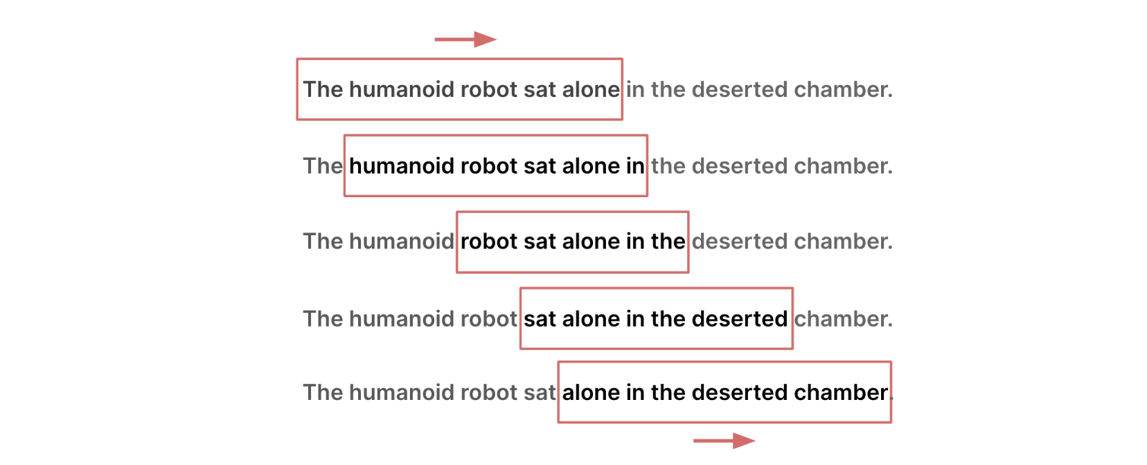
The large volume of natural language comes from internet crawling of news and articles. To turn them to training examples we use a sliding window. Starting from the beginning of the first document, at each step, the window includes a fixed number of words from within the text and these words become a single training example. The next step is taken by moving the window one word to the right in order to capture the next training example. The sliding window moves creating a training example at each step until it reaches the end of the training dataset.
 |
|---|
| Figure 9. The context sliding window. |
We can hide a certain word position within the sliding window at each step of the sliding window. For example if the window has 5 words, we can hide the middle one at each step.
 |
|---|
| Figure 10. A sliding window for masked language modeling like word2vec’s CBOW (and BERT like we’ll see in the next sections). A specific position in the window is hidden and word2vec is trained to predict it. |
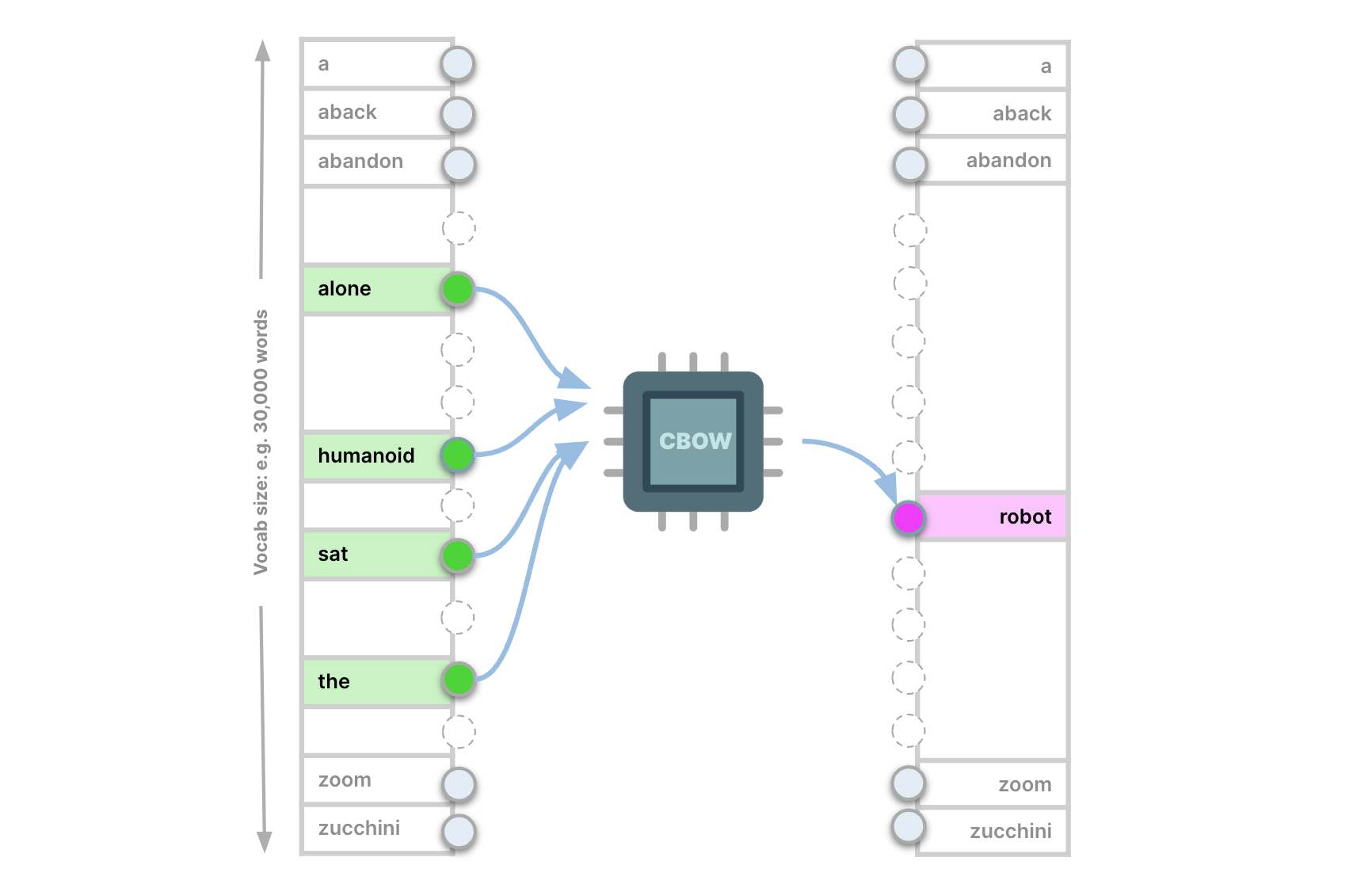
We feed the other four to the input layer of the word2vec network (in the one-hot manner that we discussed) and we use the masked word as the target for the neural network prediction. This configuration is called Continuous Bag Of Words (CBOW). To summarize, CBOW feeds the context around each word into the network and predicts the missing word, given the context.
 |
|---|
| Figure 11. CBOW receives a bag of words with a masked position and is trained to predict the masked word. |
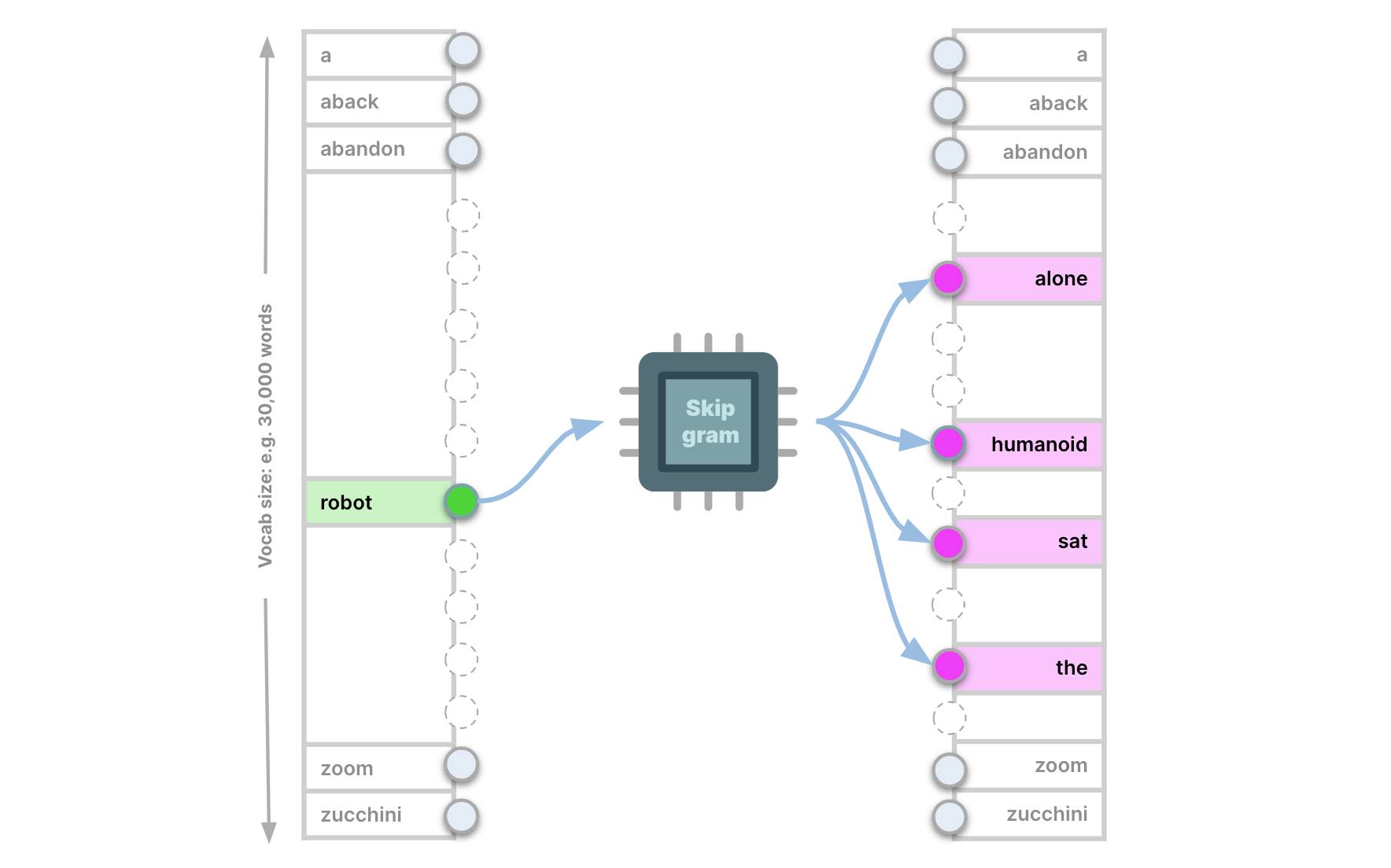
A second word2vec configuration is called skip-gram: Skip-gram hides all words in the window except one and predicts the words around it (still inside the window). So skip-gram is CBOW mirrored: we hide a certain word in the window and predict the context around it. As you probably suspect, Skip-gram performs a more challenging task: you feed it less information at each step and you ask it to predict more. Due to this, skip-gram’s language learning is deeper and its training is slower. As a result, in skip-gram, vector similarity mainly indicates semantic similarity, i.e. semantically related words obtain similar vectors. In contrast, in CBOW vector similarity mostly indicates syntactic similarity (shallower relationships, e.g. ‘dog’, ‘dogs’ etc.). The embeddings in the previous section were obtained with skip-gram.
 |
|---|
| Figure 12. Skip-gram receives a word and is trained to predict its context. |
But where do the embeddings come from in this process and how do similar words obtain similar vectors? Let’s unpack the next level of understanding of word2vec and specifically skip-gram, which is more interesting.
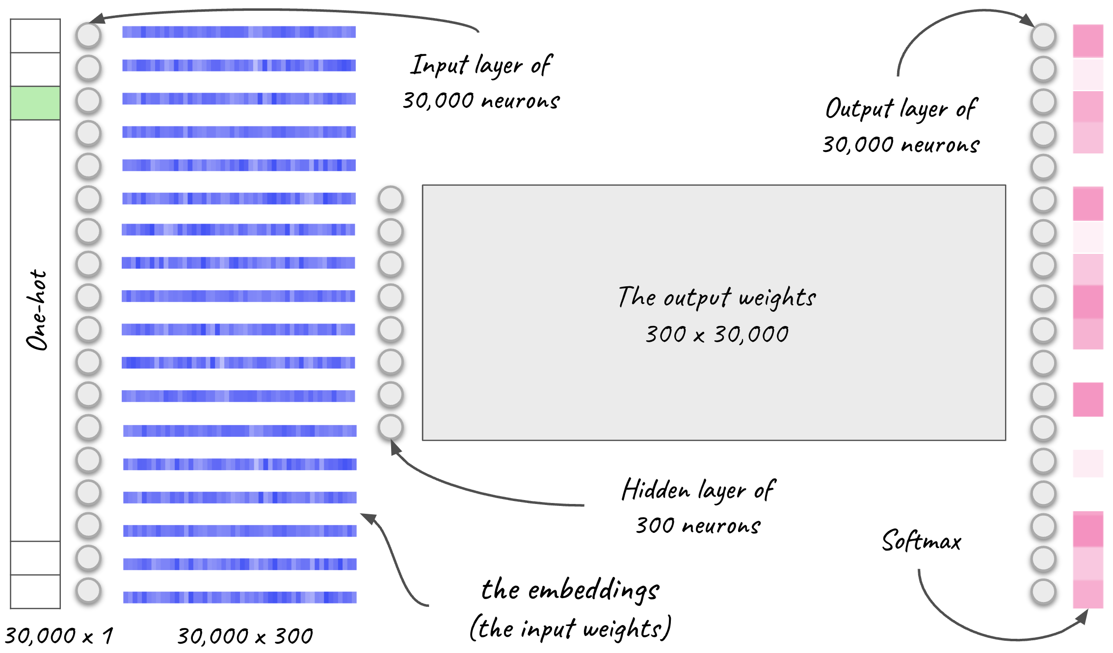
In the next image, you can see a depiction of a neural network with an input layer of size 30,000 equal to the words of the vocabulary. During training, it receives the skip-gram’s central word within a window. The output layer is a softmax that produces the probability for each word in the vocabulary to be in the context of the input word.
The hidden layer consists of as many neurons as the dimensions of the embeddings we want to learn. The embeddings we examined have 300 dimensions, so the network that produces them has a hidden layer of 300 neurons.
The word2vec embeddings, i.e. the vector for each word, are the weights of the input layer at the end of training. The hidden layer serves as a bottleneck that compresses the information into dense vectors of 300 dimensions.
 |
|---|
| Figure 13. A skip-gram neural network. The dense vector embeddings are the input weights of the network at the end of training. The vocabulary has 30,000 words and the vectors have 300 dimensions. |
Let's put everything together: Semantically related words get similar dense vectors because they have a place in similar contexts. Because, as we discussed, skip-gram predicts the most probable context for each word, this means that two semantically related words will learn to produce similar softmax outcomes. For this to happen, the corresponding input weights, which become our dense vectors for the vocabulary, have to be similar, there is no way around it.
At this point we know how the fundamental building blocks of modern NLP, the dense vectors, are computed.
The recent GenAI revolution happened with our ability to produce even more highly contextualized embeddings. Recall the old idea and quote with which we opened this section. The ability of the recent NLP engines to process context even deeper is what powered the recent advancements and superior AI capabilities. Transformers use static embeddings (such as word2vec) in the input to produce dense vectors encoding richer, more granular context.
2. Context: The bloodstream of GenAI
Generative AI and semantic AI search are the same vein and their “blood” is contextualized embeddings, i.e. the new deeper understanding of natural language, achieved by transformers. We will explain the transformer architecture in detail in the rest of this discussion.
Transformers were introduced by Google researchers in 2017 with the famous “Attention is all you need” paper [1]. The introduction of transformers was the catalyst of today’s AI boom, being the architecture for ChatGPT (GPT stands for “Generative Pre-trained Transformers”) and other viral applications.
Consider the following problems with static embeddings like word2vec:
How do we capture words that have different meanings in different contexts? For example: “Fly”: the verb vs the insect, “like”: the verb vs the preposition (“similar to”), “Apple”: the fruit vs the brand etc.
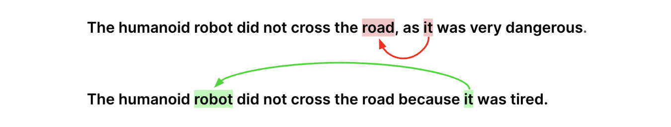
In addition, how do we deal with pronouns that refer to objects or persons? In the following example, we want “it” to be represented by a vector similar to the “robot” or the “road”, depending on the context, rather than the generic “neutral” representation of the pronoun “it”.
 |
|---|
| Figure 14. Word references. |
Enter transformer-encoders. BERT (Bidirectional Encoder Representation from Transformers) is the most prominent encoder architecture. It was introduced in 2018 and revolutionized NLP by outperforming most benchmarks for natural language understanding and search. Encoders like BERT are the basis for modern AI: translation, AI search, GenAI and other NLP applications.
With the introduction of BERT, Google achieved search breakthroughs. Today’s Google search is powered by BERT.
Understanding the context in a search query means that:
- We can surface documents that use synonyms rather than the exact query terms. And it goes well beyond synonyms by considering relevant words. As we discussed in the beginning, relevance is more powerful than synonyms alone.
- We can better understand the intent of the user: We can now attend to words that static embeddings and simple term-matching ignored. Negating words like “no” or “without” and words that involve some form of directional relationship like “to” and “for” can be very important in capturing the intent of the user and help surface the most relevant results. For example, in the query “best smartphones for photography”, the focus should be on the camera aspects. In the query “documents required when traveling from Europe to the US”, we should not surface resources discussing documents required by European countries.
- Conversely we can place less weight or ignore terms that match as part of a compound word in a document but their stand-alone meaning in a query is completely different. For example: A query including “stand” should not surface the document that you are reading despite this including the term “stand-alone”.
If you are curious to see more search examples of BERT’s breakthroughs, check this blog by Google: [2].
The same understanding of context is also what powers today’s GenAI, the two go hand in hand. In essence the interaction model changes by forming both the queries and the results in natural language rather than term-based and lists of documents. The basis is this deeper semantic understanding of natural language.
3. The transformer-encoder architecture
Think of BERT as doing fundamentally two things:
- Producing contextualized embeddings.
- Predicting a word given its context. We’ll see the details of this in the section that follows about training but fundamentally BERT is a masked language model. It can predict a masked word in a given sequence (also scroll back to figure 10).
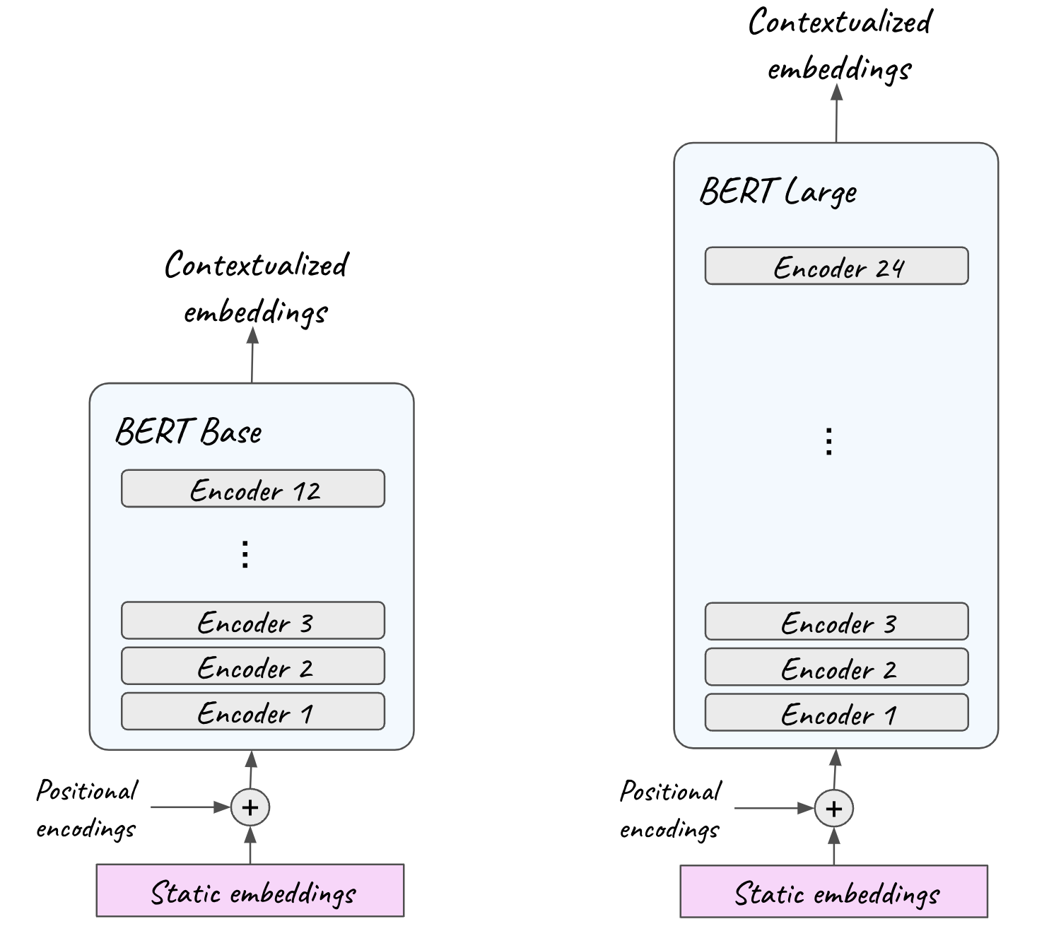
BERT receives sequences of natural language, in the form of static text embeddings (like word2vec) and outputs contextualized embeddings. Hence, we are moving from single fixed vectors for each word to unique custom representations, adjusted based on the context. BERT consists of 12 encoder blocks (24 for BERT Large) stacked one on top of the other.
 |
|---|
| Figure 15. BERT Base consists of 12 encoder layers and BERT Large of 24. They both receive natural language in the form of static embeddings, like word2vec, in the input together with positional information and output highly contextualized embeddings. |
In the input, static embeddings are coupled with positional information. Remember that during word2vec training, both CBOW and skip-gram, each sequence is treated as a bag of words, i.e. the position of each word in the sequence is neglected. However, the order of words is important contextual information and we want to feed into the transformer-encoder.
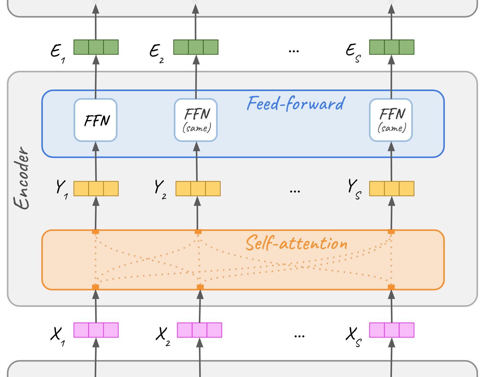
Let’s double click on an encoder block (one of the blocks out of the 12 or 24 of figure 15). Each encoder layer receives the input embeddings from the previous encoder layer below it and outputs the embeddings to the next encoder layer. The encoder itself consists of a self-attention sub-layer and a feed-forward neural network sub-layer.
The powerhouse of contextualization in the transformer architecture is the attention mechanism. In encoders specifically, it is the self-attention sub-layer. In the encoder, each sequence of natural language embeddings runs through the self-attention sub-layer and then the feed-forward sub-layer. The rest of this section will mainly unpack self-attention in detail, including why its name.
 |
|---|
| Figure 16. Each encoder layer consists, on a high level, of a self-attention and a feed-forward sub-layer. It receives embeddings from the encoder layer below it, processes them and outputs them to the next encoder layer above it. |
3.1 Self-attention
Self-attention enhances embeddings by “blending in” contextual information from within the input text. For each word in a given piece of text, it recognizes the words that are the most relevant to it in the sequence, and updates its embedding to include contextual information.
The term self-attention pertains to the ability to attend to different words within the input sequence itself (as opposed to attention systems that attend to contexts external to the input sequence, as we will see in the upcoming second part).
This way, the context influences the representation of each word and the static embedding is converted to a vector customized to the particular context. The contextualized embeddings are also dense vectors.
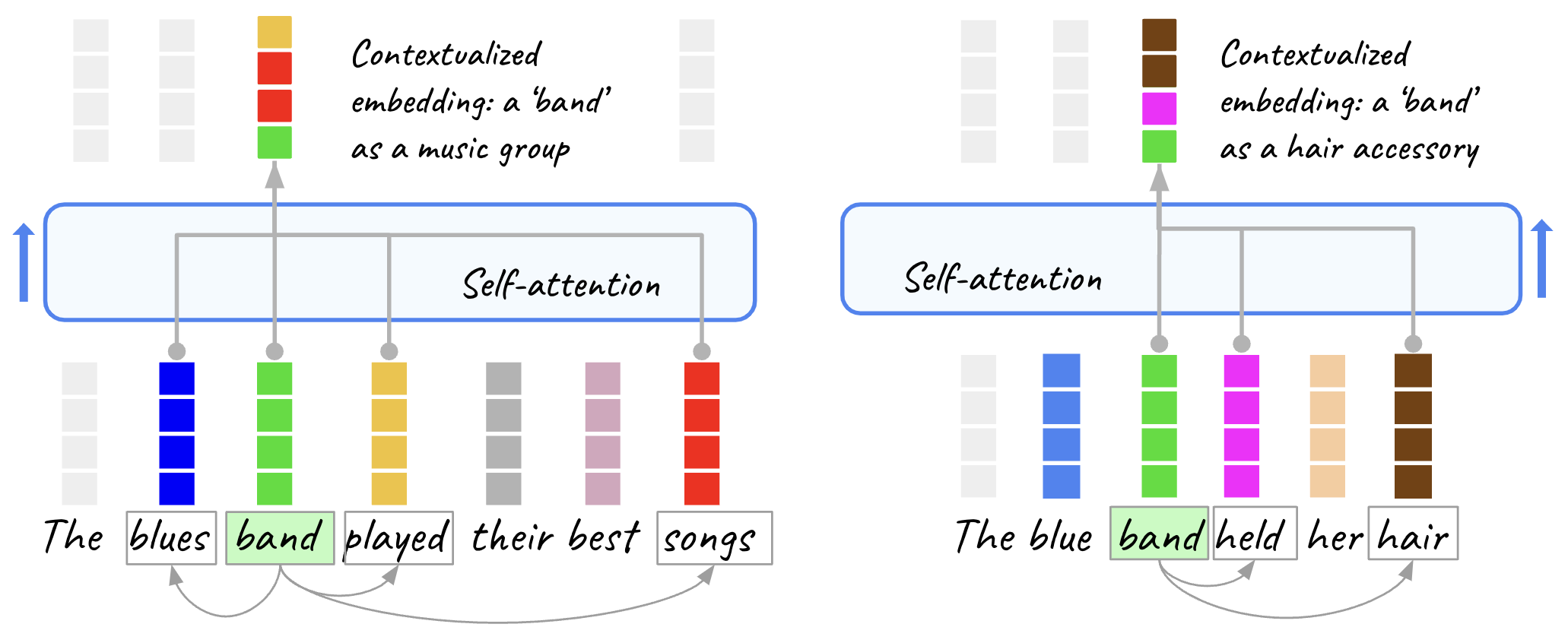
Starting from a low rigor conceptual diagram for intuition (see following figure 17), we will show step-by-step, how self-attention produces real contextualized embeddings.
 |
|---|
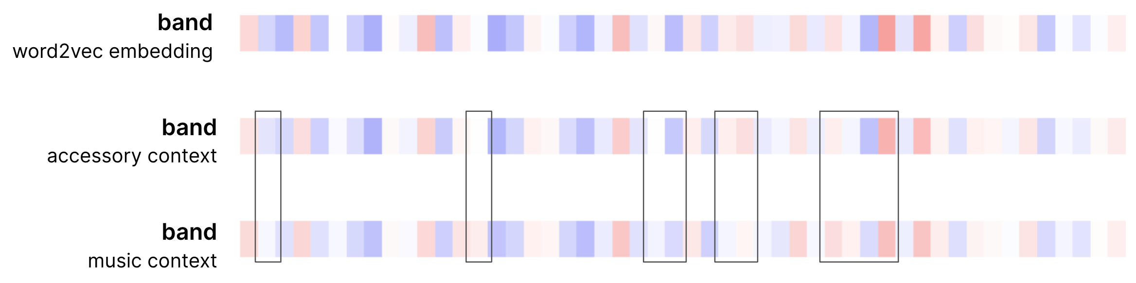
| Figure 17. "Blending" context into vectors. Self-attention disambiguates by identifying the relevant context in each sequence. In this diagram, it produces a different embedding for the same word (‘band’), depending on the context. This is a low rigor diagram, designed to illustrate a point. Continue reading and we will turn this conceptual diagram into actual contextualized representations step-by-step. |
How does it do that? With vector similarity of course: related words have similar vectors and that’s how self-attention identifies them. So for each given word X in a text, self-attention identifies the most relevant words in its context. Then it needs a way for the identified related words to influence the embedding of the given word X.
The context words influence the embedding by contributing to the contextualized vector for X. The vector for X is updated with the combined effect from the related words in its context. The more related they are, the more they contribute.
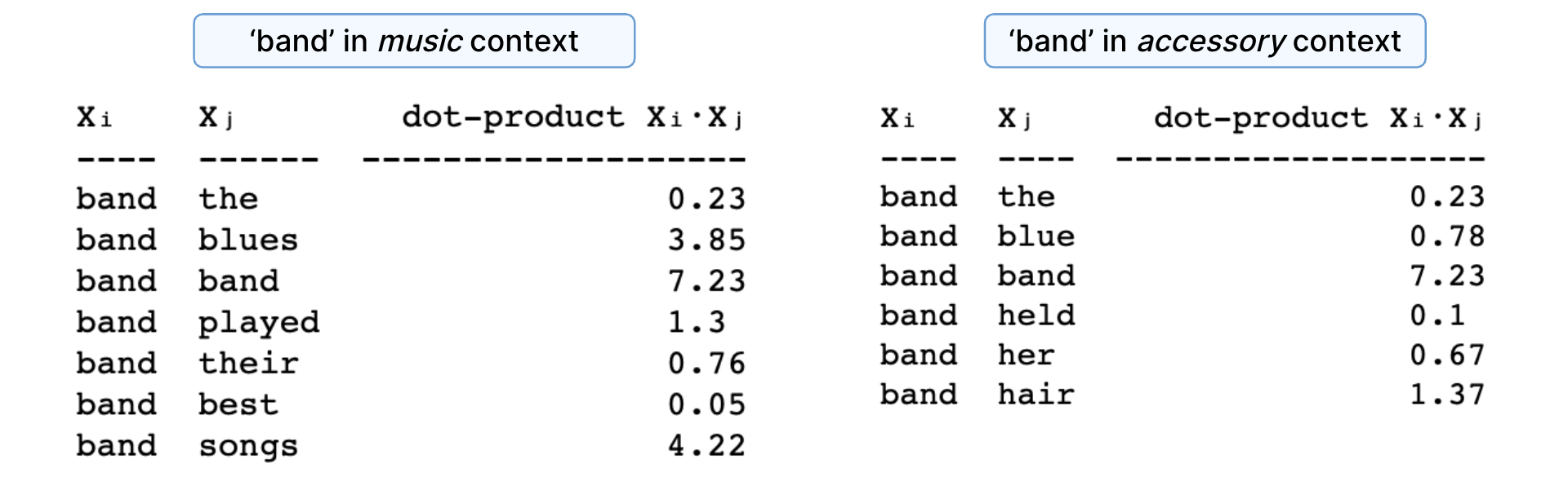
So far, we have approached vector similarity visually, now it’s time to speak to it just a little more rigorously (it’s still very simple). We’ll use dot-product as a measure of similarity. Dot-product is the sum of the element-wise multiplication of two vectors. Two vectors that are similar have a high dot-product. Two vectors that are not similar have a low dot-product.
Let’s calculate the contextual embedding for ‘band’ in two different contexts: as a music group and as a hair accessory, in the following sequences:
- “The blues band played their best songs”
- “The blue band held her hair”
First, we’ll calculate the dot-products.
 |
|---|
| Figure 18. Dot-product similarity for ‘band’ and its context vectors in different contexts, starting with their word2vec vector representation. |
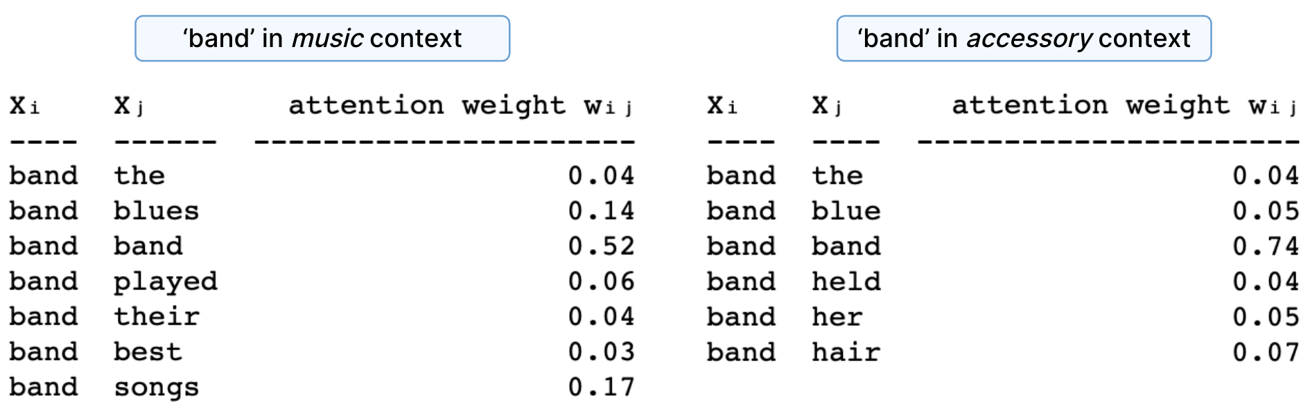
Because dot-products take arbitrary values, we normalize them to add up to 1. We do that by scaling and softmaxing. The normalized dot-products are the attention weights.
 |
|---|
| Figure 19. Attention weights for ‘band’ in different contexts. |
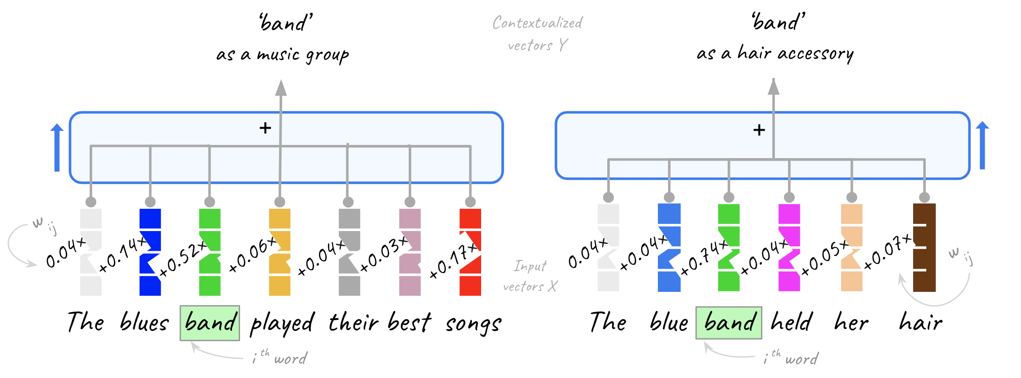
The contextualized embedding for each word is the result of adding all the vectors in the context (including itself) weighted by the corresponding attention weight. Note that the query word itself is the dominant component in the end vector, as the dot-similarity with itself produces the highest score. Intuitively, you could say that we “nudge” the original vector based on the context.
Here is what this looks like for the word ‘band’ in the previous examples, see the following figure 20:
 |
|---|
| Figure 20. Self-attention produces the contextualized embeddings as a weighted combination of the input vectors . |
The same applies to all other words in the context, we just showed it for one of them for simplicity.
So the contextualized vector for the th word in the sequence is computed as:
where is the attention weight for word and is the input vector for word .
Here is what the actual vectors look like after this operation. In this instance, we will use a three-color code (-1 is blue, 0 is white and +1 red and the real values in between are the color gradient). This choice exaggerates the differences (which are a little more subtle to easily spot with two colors) in order to help notice the effect of self-attention.
 |
|---|
| Figure 21. Visualization of contextualized embeddings (50 of 300 dimensions) for the word ‘band’ in different contexts after a single round of basic self-attention, starting from the word2vec representation. The three color code visually exaggerates the differences to help spot more easily. The rectangles highlight the dimensions that differentiate the embedding for the given word in different contexts. |
Notice that in the music example, the vector is adjusted more aggressively, as there is more relevant context and the component of the word with respect to itself receives a smaller weight (0.52 vs 0.74 in the hair accessory example).
We now have two different representations for the same word, depending on the context. Now you know the basic mechanics of self-attention.
At this point, you are either already satisfied or you are already thinking:
“Hang on a sec. The vectors for the two entirely different meanings of ‘band’ are so similar that you had to highlight the differences. Why?”
Good catch! First, notice that the input we worked with was static word2vec embeddings, i.e. we virtually worked on the bottom encoder layer. Recall that BERT has 12 encoder layers and BERT large has 24. Each layer changes the embeddings further. Second, we haven’t yet included in our narrative the second sub-layer within the same encoder block: the feed-forward network (we’ll discuss it next).
And that’s not all. The core mechanism we discussed is enhanced in two more ways for self-attention to be able to deploy its full power that you witness in Google search, Elastic’s AI search and generative AI applications.
So the third point is that the self-attention system that we have discussed so far has not introduced any learned parameters. So far, all values are computed based on the existing vectors. A learning system requires parameters that are learned during its training, in order to generalize.
For this purpose, self-attention employs a system of parameter matrices and operations on them. We will not go into the details because they are not incredibly fun but because it is very likely to get confused at this point when reading other resources, we will describe the gist of it here. Feel free to skip this point (certainly don’t hang on it):
We have the opportunity to introduce parameters at the following points of the self-attention operations that we have described so far:
- When calculating the dot-product, we can parameterize vector and vector . We introduce an independent parameter for each position of these vectors. You will come across the following terminology at this point: we call the vector that results from the parameterization of vector (the sequence position that we are looking to produce its contextualized embedding for) the “query” vector. We call the vectors for the words in the sequence that result from the parameterization of vectors the “key” vectors.
- When calculating the contextualized embedding by multiplying the attention weight (as a result of the previous step) with the vector for each position and then summing for all positions of the sequence. We parameterize with new variables (independent of the ones we gave it in the previous step). In self-attention terminology we call the parameterized versions of vectors for this step, the “value” vectors.
Introducing these parameters and learning them during training the encoder, optimizes the creation of contextualized embeddings.
And then there is multi-headed self-attention.
3.2 Multi-headed self-attention
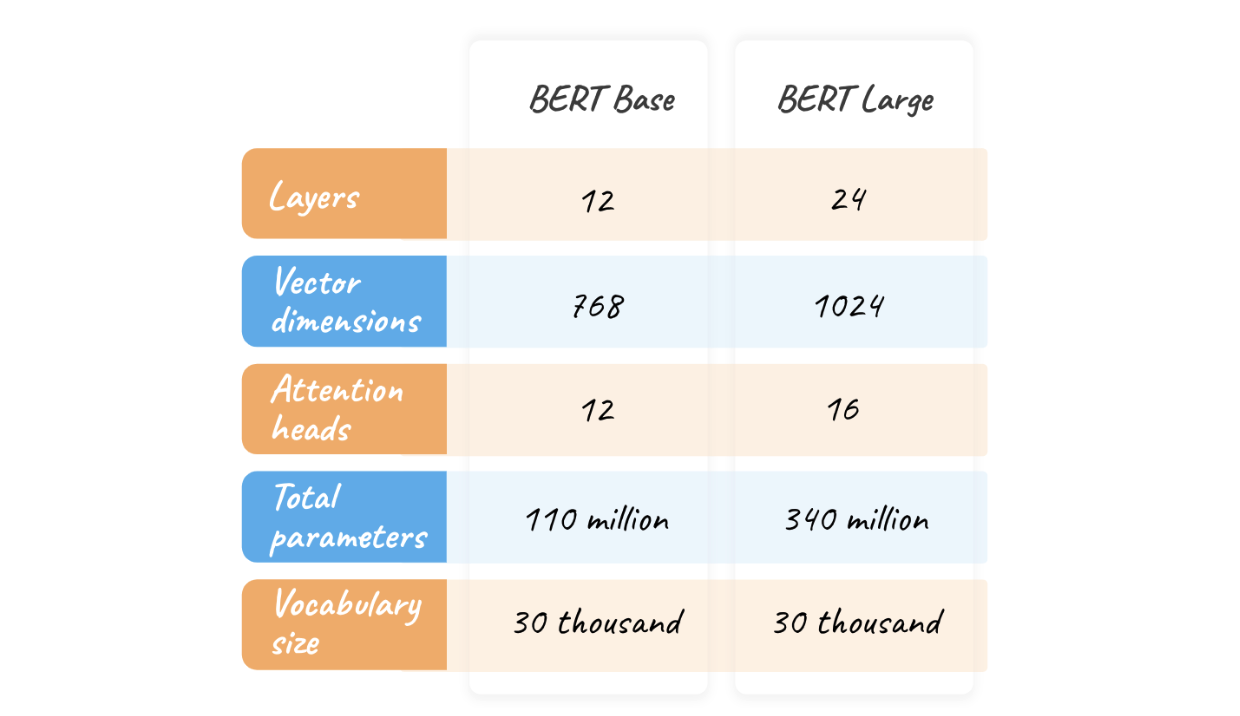
The parameters we just talked about are a fundamental part of the architecture, because without them self-attention would not be the learning system that it is at the heart of a language model. One step further, we enhance it with even more degrees of freedom: more parameters to be learnt in parallel. We are building a large language model after all and “large” means hundreds of millions of parameters (BERT has roughly 110 million parameters, BERT Large roughly 340 million parameters and GPT-3 roughly 170 billion parameters) and we can do that because we train it on huge corpuses.
Here is why we want to do this: Consider input texts longer than the toy sentences we’ve played with so far. The longer the context, the weaker the influence of the relevant words towards a contextualized embedding (think of the normalized attention weights, the more the words, the smaller each one’s influence).
To mitigate this, we replicate the mechanism we have described so far by executing it multiple times in parallel using independent parameters within what is called a self-attention head. As a result, we multiply the parameters we just introduced by the number of self-attention heads. Each head executes the algorithm that we have described so far, independently of all others. BERT Base in particular deploys 12 attention heads (and BERT Large 16).
With one head, self-attention may or may not be able to focus on the relevant terms in long sequences. Multiple heads just do it.
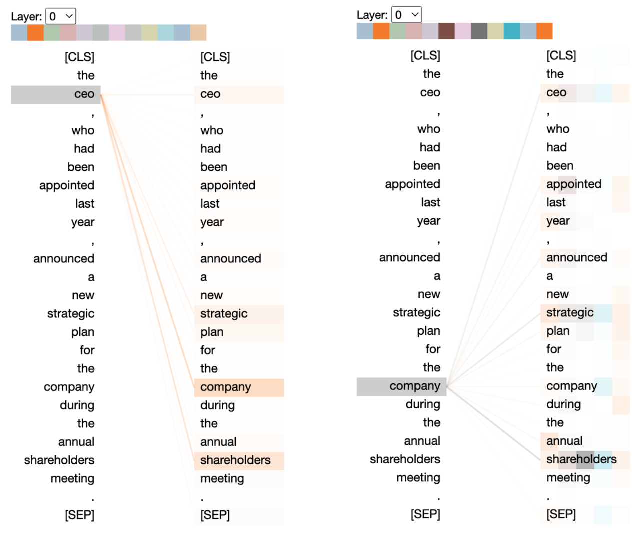
Let’s move from our introductory setup on to visualize actual BERT’s multi-headed self-attention using Bertviz. In the following visualization, each head is represented by one of the colors in the array at the top. The connectors show the relationships that each head focuses on. In the self-attention terminology we introduced earlier, the left column is the “query” vector to examine which “keys” it focuses on from the right column (the same sequence is shown in two columns for a clearer visualization of self-attention). The more intense the color, the higher the attention weight.
 |
|---|
| Figure 22. Visualizing long-range relationship understanding with self-attention in BERT. Created with Bertviz. |
There are a few interesting things to notice.
Multi-headed self-attention is able to capture long-range relationships (the example is suitable to exhibit such relationships). Notice how in the second self-attention head (orange) ‘ceo’ attends to ‘company’ and ‘shareholders’, both several words away. Similarly, for ‘company’, multiple heads attend to ‘shareholders’ and ‘strategic’, all several words away. This is noteworthy because previous technologies were not able to capture such long-range relationships effectively.
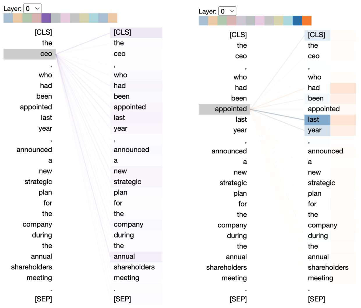
Contrast this behavior with the 5th head (with purple on the left in the next visualization). It misses important relationships for ‘ceo’, suffering from the loss of focus effect that can happen in long sequences like we discussed. The multi-head added value is appreciated here, as a single head may be stuck in a behavior like the 5th head’s.
 |
|---|
| Figure 23. On the left: Understanding the value of multi-headed attention. A single head… misses the point in a long sequence. As influence disseminates evenly, the head loses the right focus. On the right: capturing other linguistic relationships. Created with Bertviz. |
In addition, notice how on the right visualization self-attention is able to capture other syntactic relationships, like temporal information for the verb ‘appointed’ (although this is more debatable as these words are in the proximity).
There is active research around multi-headed self-attention and the extent to which it can (or cannot) capture syntactic/linguistic phenomena. If you are curious, the “What Does BERT Look At?” [3] and “Assessing BERT’s syntactic abilities” [4] papers are good starting points. Their authors analyze how self-attention captures different language relationships such as the ones of direct objects to their verbs, noun modifiers to their nouns, propositions to their objects etc.
Finally, notice that each head calculates its own contextualized embedding for each word of the input sequence. However, the encoder outputs one embedding for each word, so we need a way to combine the output from each head to a single one. At this point you will not be surprised that to do so, we introduce more parameters to the model, whose role is to create the right combination.
3.3 The feed-forward neural network
The second component within each encoder layer is a feed-forward neural network (FFN for short), refer to figure 16. This is a fully connected neural network which is applied to each position of the sequence. In the original transformer architecture, the dimensionality of the inner layer of the FFN is four times the dimensionality of the embeddings, which in turn is 768 for BERT Base, 1024 for BERT Large and 512 for the full transformer.
The first thing to note is that while in the self-attention layer the input embeddings in a sequence interact with each other to produce the output of the sub-layer, they go through the FFN sub-layer in parallel independently.
The second thing to note is that the same FFN, i.e. an FFN with the same weights, is applied to each sequence position. This is the reason why it is referred to as a stepwise FFN in the literature. However, while the FFN has the same weights across the positions in the same encoder layer, it has different weights across the different encoder layers.
Why these choices? Of course, having different FFNs across the different layers allows us to introduce more parameters and build a larger and more powerful model. On the other hand, the reason why we want the same FFN in the same layer is less obvious. Here is an intuition: If we feed a sequence of the same repeating embedding (e.g. the same word) in the FFN sub-layer, the output embedding of the sub-layer should also be the same across all positions of the sequence. This would not be the case if we allowed multiple FFNs with different learnt weights in the same sub-layer.
With the architecture clarified, and with the role of self-attention being to synthesize contextualized embeddings, the next big question is: What is the role of the FFNs in transformers?
On the highest level, note that the self-attention sub-layer, as we described it in the previous sections, only involves linear transformations. The FFN sub-layer introduces the non-linearities which are required in order to aim to learn optimal contextual embeddings. We will attempt to approach closer what this means in part-2 of this post, in the context of the full transformer architecture by unpacking some of the intuitions offered by the research conducted in this active area.
Let’s wrap up this section by summarizing the BERT architecture:
 |
|---|
| Figure 24. Overview of BERT Base vs BERT Large architectures. |
4. Training and fine tuning language models for AI search and NLP
We’ve seen how transformer-encoders and BERT work, it’s time to examine their training in more detail.
Training involves learning all these parameters that we have discussed in the self-attention and feed-forward sub-layers (see figure 16) and, as discussed, is based on masking (see figure 10): The encoder is presented with a vast corpus. In each training sequence, words may be masked.
BERT specifically is trained on the entire Wikipedia and BookCorpus by masking 15% of the input and asking it to predict the masked words. 15% is the sweet spot between too much masking, which makes training very expensive, and too little masking, which removes useful context during training.
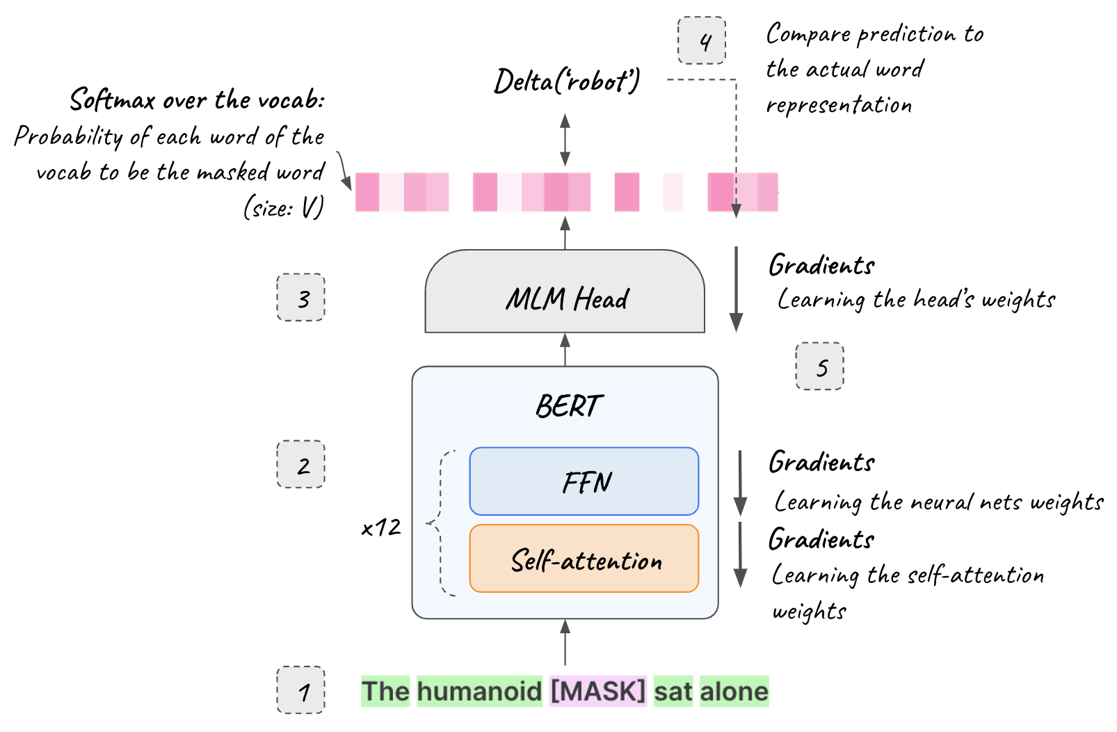
For training we use a masked language model “head” (MLM for short) at BERT’s output. The MLM head is the neural network that predicts the masked word. It has as many input neurons as the number of possible words in BERT’s dense input (768 for BERT Base) and as many output neurons as the words of the vocabulary. For each masked sequence during training, the head receives the contextualized embeddings for the sequence (BERT’s output) and produces the probability of each word in the vocabulary to be the masked word (the typical softmax is used).
The delta between the prediction and the actual word representation is calculated and the gradients backpropagate throughout the whole architecture, adjusting the values for each encoder’s self-attention and feed-forward network sub-layer parameters that we discussed in the previous sections (as well as the head itself). Reference [5] is a refresher of backpropagation (as stated in the beginning, we assume that you are familiar with the neural networks fundamentals).
After training, we discard the MLM mask and the encoder is ready to produce contextualized embeddings for any input sequence.
 |
|---|
| Figure 25. Masked language model training: 1. The masked sequence input. 2. The sequence goes through the 12 encoder blocks in this BERT Base example. 3. The MLM head produces the prediction of the masked word as a probability distribution over the vocab. 4. The actual word (“robot” in this example) representation is presented and the delta calculated. 5. The gradients backpropagate, adjusting the weights throughout the architecture. |
4.1 Training patterns and language model transfer learning
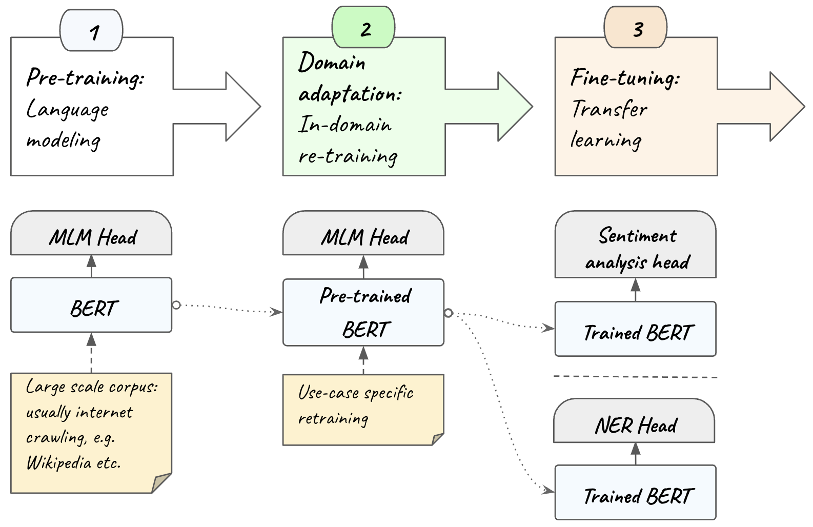
On a high level, training a model involves three phases:
Pre-training: The architecture is trained as a masked language model on a large dataset, with an MLM head, like we have seen so far. The advantage of the approach is that using masking with tactics like the sliding window, we can pretrain the model without the need of any labeled data.
Domain adaptation: For the best results, we retrain the pretrained model on in-domain data. For this we must use a corpus from the target domain, i.e. the subject area or field of knowledge that the model will be used in, in order to help it pick up the terminology and language patterns of the specific domain. We may have a smaller corpus of in-domain data but the fact that we have pre-trained the model on a large corpus allows it to perform well after in-domain retraining. Domain adaptation can also be done with an MLM head, without tagged data.
Fine-tuning: Except for search, encoders like BERT are used for many NLP tasks including sentiment analysis and other text classification, named entity recognition (NER), question answering etc. In the last phase, we employ a task-specific head on top of the transformer-encoder, designed for the particular task at hand. For example, for a sentiment analysis task, the head is a small feed-forward neural network that is trained to output the probability of each class. In this stage the encoder is used as the feature extractor: It produces the contextualized embeddings that are used as the input to the NLP Head. This tactic is called transfer learning and it has been applied for training computer vision models before applied to NLP. This stage requires labeled data.
 |
|---|
| Figure 26. Transfer learning. |
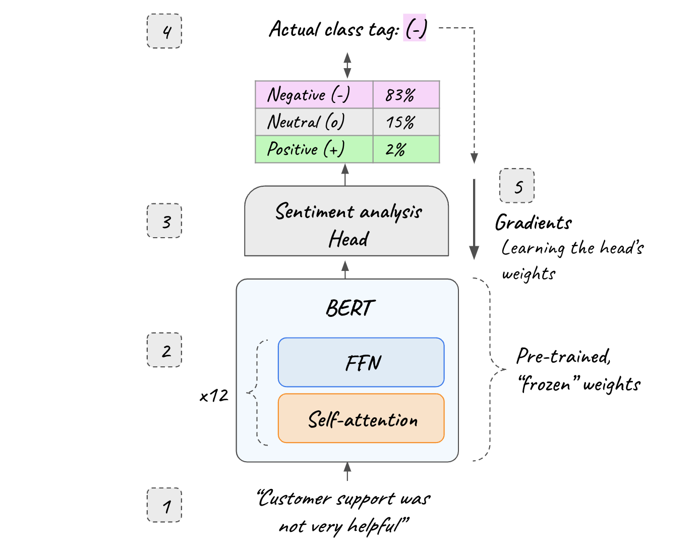
Note that with transfer learning, we can use a pre-trained transformer-encoder to just train the text classification head on top of it. This greatly simplifies the Machine Learning work that we need to do compared to choosing to adjust the weights throughout the entire architecture during training. In practice, this means taking an existing pre-trained BERT model, “freezing” all its parameters, adding an output layer to it, and training only the last layer to the task at hand. This way, we only need to adjust the last layer's weights, as opposed to the hundreds of millions of weights that BERT contains. Transfer learning is very powerful, as by freezing BERT’s millions of parameters, the training time, resources and in-domain data requirements are greatly relaxed.
 |
|---|
| Figure 27. Transfer learning for sentiment analysis based on a pre-trained BERT. Contrast this pattern with the end-to-end training of figure 25. |
Elastic Machine Learning makes it extremely easy to upload and deploy the supported pre-trained transformer-encoder NLP models from HuggingFace or your custom models from your environment to use with your Elastic data.
4.2 The AI barrier
Training, in-domain adaptation and fine-tuning language models present a material barrier: They require significant human and computing resources: On one hand, machine learning expertise requires scientific talent well beyond conventional software engineering. On the other hand, training models is resource intensive, often requiring GPU hardware and several weeks or months of processing time, all of which have significant cost.
And that’s far from the whole picture: you also need validating and testing your models offline and online before deploying them to production.
Fine tuning requires tagged data, which means that you either need to spend manpower on or outsource your data labeling or to produce systems that can automatically label your data with very high accuracy.
Your production data pipelines may need to change significantly in order to accommodate preprocessing data for training. And in addition If your production data are not synced with your test environment data, as it is often the case, this may cause even deeper data engineering and operations effort.
Furthermore, models and data are not static, you will probably need to build model drift and data drift detection to mitigate any training-serving skew.
Because of the special hardware and software requirements there is a good chance that your MLOps will probably require a different release cycle than the rest of your software. You will need to build the appropriate integrations with the rest of your software.
For all these reasons and more, AI-powered natural language understanding and search present a very high barrier for most organizations.
5. Elastic Learned Sparse Encoder for AI search out of the box
Elastic Learned Sparse Encoder (ELSER) solves this for the search use case. It builds on BERT to provide superior AI search out of the box [6]. You can download ELSER and deploy it with just a couple of clicks from within the Elastic UI. ELSER requires truly zero ML effort: It relieves you entirely from the AI barrier briefly described in the previous section. it also requires no external component to start using it with the familiar Elastic search APIs.
With this, Elastic now offers two options:
- Its own out of the box, proprietary AI search model.
- Deploying third party vector models for use with Elastic data.
Here is how ELSER works.
As we discussed, after pre-training (and domain adaptation if one is performed), we generally discard the MLM mask as the encoder’s main purpose is to produce contextualized embeddings for any input sequence (if our use case does not involve task-specific fine-tuning).
However, at the end of the training process, the MLM head is a trained neural network which produces a probability distribution over all the vocab, for each masked input term (contextualized because BERT is doing its magic under the hood) within any input sentence.
In the search use case, the input sequence is our query. Each position of the input sequence/query produces a different such distribution over the vocab, by activating different words in different degrees.
The idea behind ELSER is instead of discarding the MLM head, to use it in order to produce these distributions for each word in the sequence/query. Because the MLM head is not sparse by design, we modify it appropriately and adapt the training objective to make it sparse and optimized for retrieval.
If we aggregate the per-word distributions into one for the whole sequence/query, we are producing a vector, the values of which represent how much each word in the vocabulary is activated by the input query.
 |
|---|
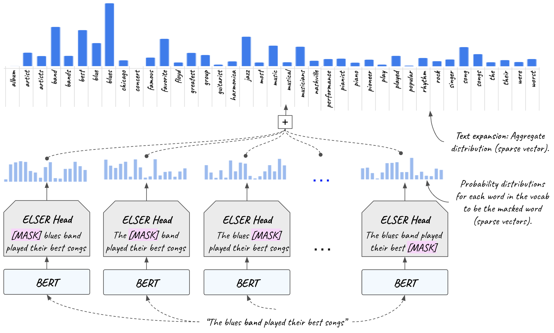
| Figure 28. With Elastic Learned Sparse Encoder the “the blues band played their best songs” query gets expanded to a sparse vector of relevant words (“album”, “artist”, “concert”, “favorite”, “jazz” etc.) with the use of ELSER’s MLM. The vector (at the top of the figure) is sparse, containing a position for each word in English and its corresponding relevance score to the query (depicted as a histogram). The vast majority of them are zero and they are omitted for visualization purposes. |
Because this vector is of size equal to the size of the vocabulary and the activated (non-zero) dimensions are a small fraction, it is a sparse vector.
We then perform search not only based on the query terms, but also using the activated words from the entire vocabulary. This capability is called text expansion. Text expansion refers to the ability of surfacing semantically relevant documents in search results even if the query terms are not present in the documents. Think of it as “expanding” the query beyond the exact search query terms that are used, to activate relevant terms that exist in the documents but do not exist in the query itself. This is known as the vocabulary mismatch problem and ELSER mitigates it.
Figure 28 shows text expansion with ELSER in action. The input sequence (“the blues band played their best songs”) activates relevant words in the English language (e.g. “album”, “artist”, “concert”, “favorite”, “jazz”, “piano” etc.). ELSER’s MLM head is used to expand the query.
The expanded query is then used for search in place of the original shorter query. The vector is sparse, containing a position for each word in English and its corresponding relevance score to the query.
 |
|---|
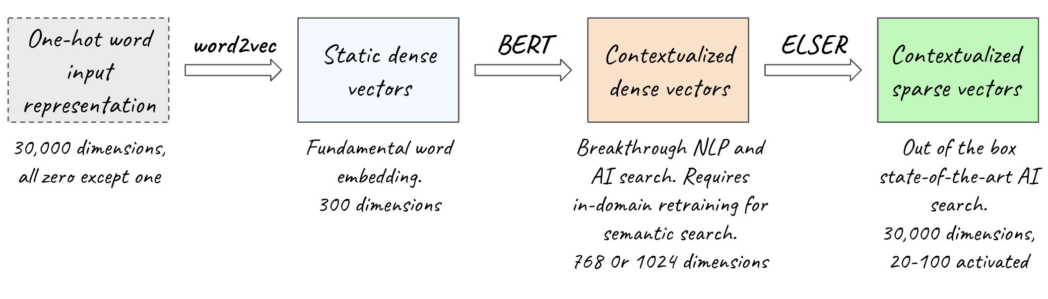
| Figure 29. Overview of how the models and representations covered in this article relate. |
Text expansion is more powerful than using synonyms because it can rank results based on a granular “relevance continuum” on the language-level and scale, rather than on the document corpus level with synonyms used in combination with the conventional term-based TF-IDF.
Elastic Learned Sparse Encoder is state-of-the-art: it outperforms both simple term-based search (BM25) and dense vector semantic search when no domain adaptation is performed, it is the best model for out of the box AI search at this point [7].
Because it produces sparse contextualized vectors, you can use it out of the box with the familiar Elastic search APIs without any Machine Learning expertise or MLOps effort. For the same reason and because of Elastic’s vector database capabilities, it is also more resource efficient than dense vectors having a smaller RAM footprint.
Deploy it with one click from the Elastic UI and start leveraging AI search’s superior relevance, as we explained it in “the bloodstream of GenAI” section.
Conclusion
We hope that this post helped you build a good understanding of AI language models and the intuitions behind the breakthrough architectures. So congratulations, you came very far and you now know everything you need in order to understand generative LLMs, which will be the topic of the second part of this article. You have completed the hardest part, tune in.
References
- Attention is all you need
- Understanding searches better than ever before
- What does BERT look at? An analysis of self-Attention
- Assessing BERT’s syntactic abilities
- How the Backpropagation algorithm works
- Elastic Learned Sparse Encoder: Elastic’s AI model for semantic search
- Improving information retrieval in Elastic